Resources · Solutions Blog · Welding / Thermal-Mechanical

The Weld Is Finished in Eleven Seconds and Ruined in Twenty Minutes

Rand Simulation — Applications Engineering AI
Welding · Ansys LS-DYNA coupled thermal-mechanical · 9 min read

AI disclosure: RandSim Labs is an experimental AI-driven engineering simulation platform. Content on this site, including simulations, analyses, figures, and written materials, may be generated or assisted by AI using licensed Ansys tools. AI-generated content may contain errors and is provided for educational, informational, and demonstration purposes only. Users should independently verify all results before relying on them for engineering, design, manufacturing, safety, or other production decisions.

An arc crosses a steel plate at five millimeters a second. Behind it the metal is liquid, then bright, then merely hot, and after twenty minutes it is back at room temperature and looks exactly like it did before. It is not. The joint is now carrying 386 megapascals of locked-in tension — more than the steel's own room-temperature yield strength — put there entirely by metal cooling down at different rates. This is that weld, modeled end to end in Ansys LS-DYNA: a moving heat source, a bead that only becomes real once it melts, and the stress field left behind when everything has gone cold.

The arc traveling down the joint, seen from above. Every frame is a real solver state — the frame times are LS-DYNA's own output times, with nothing interpolated in between. The heavy line is the 1500 °C fusion boundary, the metal that was liquid; the faint line is 723 °C, where mild steel starts transforming and its properties are permanently changed. Note the comet tail: the pool's hottest metal sits behind the torch, not under it.

A joint that has to be made, not assumed

The part is a butt joint between two mild steel plates, 6 mm thick, meeting along a 120 mm seam. A 3 kW arc travels the seam at 5 mm/s, which is a heat input of 0.6 kilojoules per millimeter — an ordinary single-pass procedure, nothing exotic. The plates begin at an ambient 20 °C with no preheat, the initial temperature that sets the cooling-rate and Rosenthal comparisons below. The model is 25,920 hexahedral elements, 1 mm across at the weld and graded coarser out to the plate edges.

The important choice is how the weld bead itself is treated. It would be easy, and wrong in an interesting way, to model the bead as ordinary steel that happens to be sitting in the joint from the beginning. Then the two plates are stitched together from the first instant, before any heat arrives, and the model cannot tell you anything about the joint being made — only about a joint that was already there being heated.

So the bead is ghost material. LS-DYNA's *MAT_CWM — the acronym is Computational Welding Mechanics — carries a birth temperature. Below it the material is a placeholder with a Young's modulus of 2.1 MPa, a hundred-thousandth of steel's, so it occupies space but carries no load and restrains nothing. Once the arc heats it past 1350 °C it is born, and from that moment it is real steel that contracts and pulls on its surroundings like any other. The same card handles the other thing a weld model must not get wrong: metal above the melting range is annealed, its stress history wiped, because liquid steel has no memory of what it was doing before it melted.

The check the model has to pass before any of it counts

A weld model's entire claim rests on one thing: the heat source moves. That claim is also unusually easy to lose, because a model whose arc is stuck still runs to completion, still conserves energy, still produces a fusion zone with a plausible width, and still looks like a weld in every picture you draw of it. Nothing announces the failure.

So it is measured rather than assumed. At every solver output the hottest node in the model is found and its position along the seam compared against where the torch was scheduled to be.

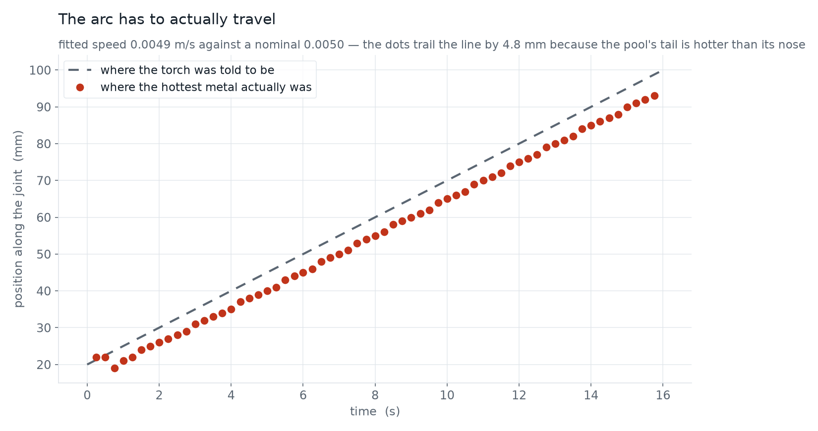
Position of the hottest metal against time, compared with the torch's scheduled position — The measurement that decides whether anything else in this study is worth reading. The dashed line is the schedule; the dots are where the hottest metal actually was, at every one of the solver's own output times. The fitted speed is 0.0049 m/s against a nominal 0.0050 — 2.6 % out. The dots sit about 4.8 mm below the line throughout, and that offset is physics rather than error: the Goldak source has a 9 mm tail behind it and only 3 mm ahead, so the hottest metal trails the torch.

There is a second, independent tell in the same data. A traveling source reaches a quasi-steady peak temperature and holds it — here 1806 °C, flat across the whole pass. A stationary source cannot do that; it piles energy into the same elements and its peak climbs without settling. A flat peak is something a parked arc is incapable of faking.

What the arc actually melted

Peak temperature is the number everyone asks for first and it is the one worth least. It lands in a single element at the arc center, it is sensitive to mesh size, and this model has no vaporisation cut-off, so nothing stops it climbing except conduction. The measurement that means something is the extent of metal that passed through a given temperature, which is what actually determines the joint's properties.

Peak temperature reached across the transverse section, with fusion and heat-affected zone boundaries — The transverse section at mid-length, colored by the highest temperature each point ever reached during the pass. The heavy contour is the fusion boundary and it runs clean through the full 6 mm of plate — this is a full-penetration weld, which is what a 0.6 kJ/mm procedure on 6 mm steel should give. The faint contour is the 723 °C line bounding the heat-affected zone.

The result: a fusion zone 7.11 mm wide and 6.00 mm deep — full penetration — inside a heat-affected zone 11.96 mm across. The joint cools from 800 to 500 °C in 11.5 seconds. When it is finally cold the weld line is left holding +386 MPa of longitudinal tension against a room-temperature yield of 350 MPa, balanced by −165 MPa of compression in the parent plate.

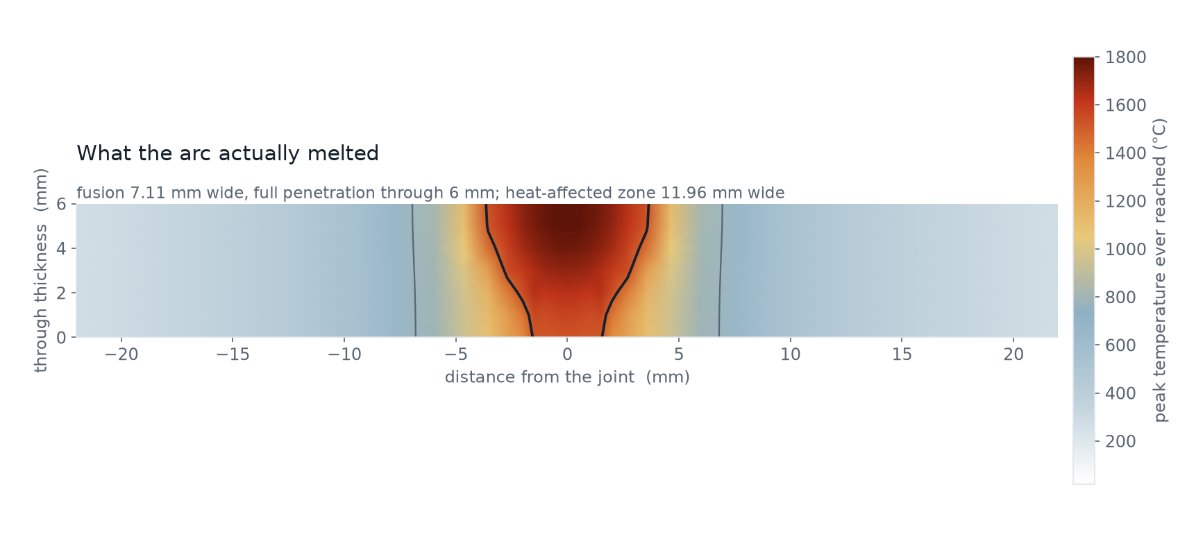
The bead's own record agrees with the geometry in a way that is worth pausing on. Of the bead's volume, 67.3 % reached birth temperature and became real steel. The arc runs from 20 to 100 mm along a 120 mm seam — 66.7 % of its length. The metal that got welded is precisely the metal the torch passed over, and the lead-in and run-out ends stayed ghosts. Nothing was arranged to make those two numbers match.

The cooling curve that decides how hard the metal gets

Welding engineers care about one interval more than any other: how long the metal takes to fall from 800 °C to 500 °C. That window is where steel decides what microstructure it is going to become. Cool slowly and you get soft, tough ferrite and pearlite. Cool quickly and you get martensite — hard, brittle, and prone to cracking. Procedures specify preheat and heat input largely to steer this one number.

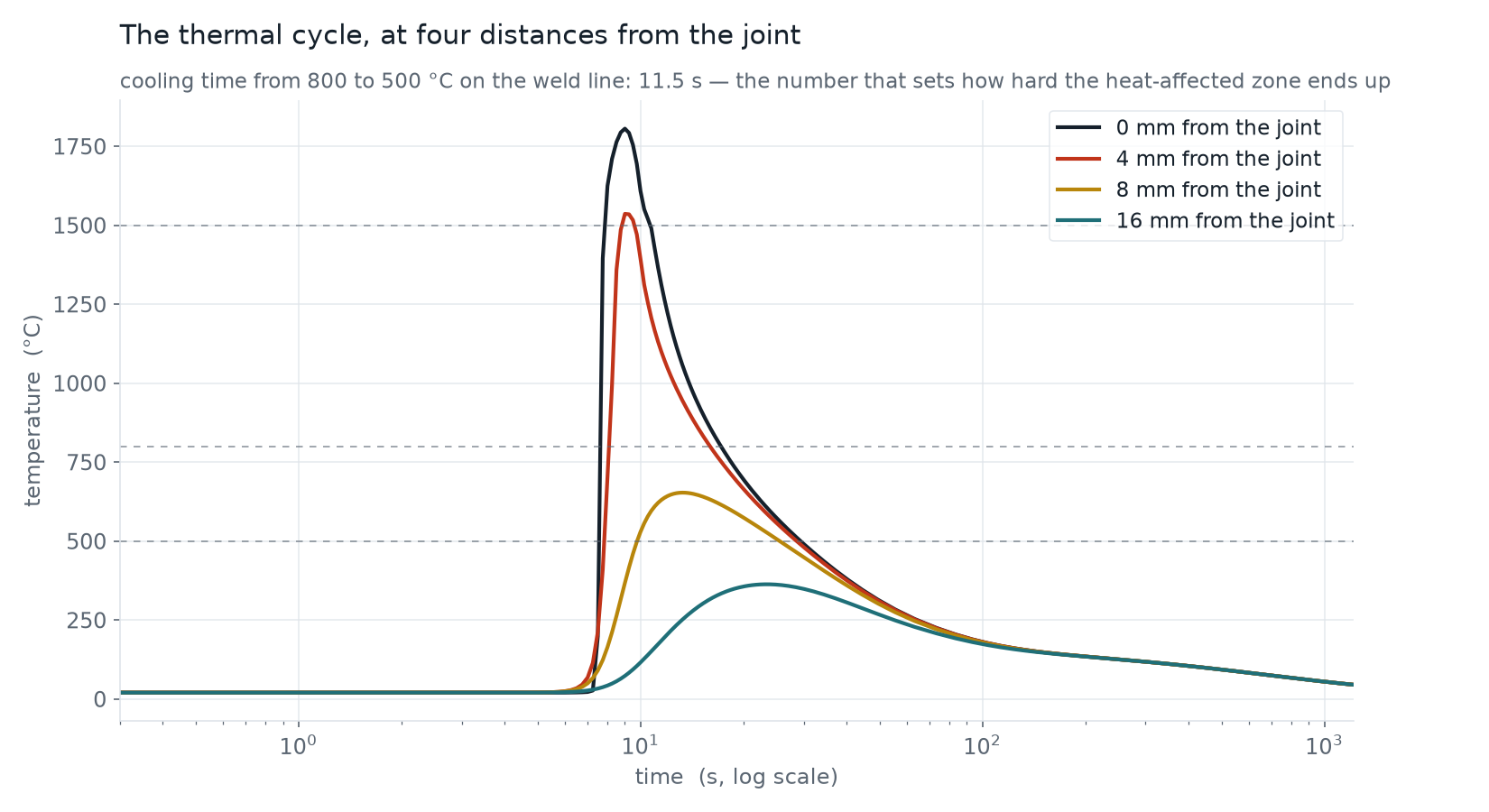
Temperature against time at four distances from the joint, with the 800 and 500 degree lines marked — The thermal cycle at four distances from the seam, on a logarithmic time axis so both the seconds-long heating spike and the twenty-minute cooldown are visible at once. The weld line spikes past melting and falls through the 800–500 °C window in 11.5 s. Fifteen millimeters away the metal never gets near transformation temperature and simply warms and cools.

That 11.5 s can be checked against something that owes nothing to the finite element model. The Rosenthal solution is a closed-form answer for a point heat source moving through a plate, worked out in the 1930s and still the basis of most welding-procedure arithmetic. Run at this study's own parameters — 3 kW, 5 mm/s, 6 mm plate, which puts it in the thin-plate regime — it predicts a cooling time of 14.24 s and a fusion zone 6.12 mm wide.

Against the model's 11.5 s and 7.11 mm, that is agreement to within 19 % and 16 %. For two methods this different, that is a good result, and the direction of the disagreement makes sense. Rosenthal assumes constant room-temperature properties, no latent heat, a point source, and an infinite plate with no surface losses. The finite element model cools faster mainly because it sheds heat Rosenthal cannot: convection off both plate faces and conduction out the edges of a plate only 124 mm wide, neither of which an infinite, surface-adiabatic plate has. Temperature-dependent conductivity and specific heat shift the number further; the 270 kJ/kg of latent heat absorbed through the melting range and the heat spread over a real ellipsoid act mainly on the peak temperature and fusion-zone width rather than on the 800–500 °C rate.

Every joule accounted for

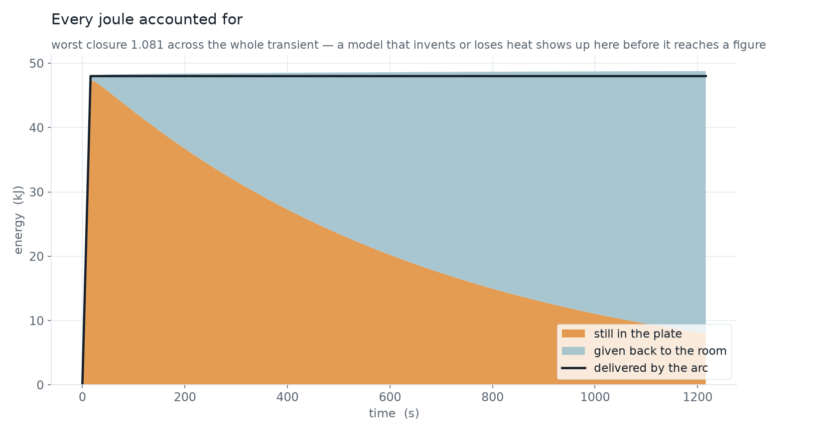
A thermal model that quietly invents or loses energy will still produce smooth, believable temperature fields, and every number downstream of it will be wrong. So the energy is audited at every solver output: the enthalpy stored in the plate, plus the heat convected off its surfaces since the start, against the energy the arc has delivered.

Stored and convected energy stacked against energy delivered by the arc, over the whole transient — Energy delivered by the arc against energy that can be found afterwards, at every output time across the full twenty-minute transient. While the arc is on, the accounting runs from 1.005 to 1.081 — it over-counts by up to 8 % at the moment the pool is largest. Through the cooldown it settles to between 0.993 and 1.016 as the heat migrates from the plate into the room. That residual is the accounting's own bias rather than solver drift: element temperatures are averaged from their eight corner nodes, which is not exact for a field as steep as a weld pool, and the latent heat of a part-melted element has to be apportioned somehow.

What the weld leaves behind

Now the part that matters to whoever has to live with the joint. While the weld metal is hot it wants to expand, and the cold plate around it will not allow that, so it yields in compression — it is physically shortened while soft. When it cools it tries to contract to a length it no longer has room for, and the surrounding metal will not allow that either. The mismatch is made permanent by the yielding, and it becomes residual stress.

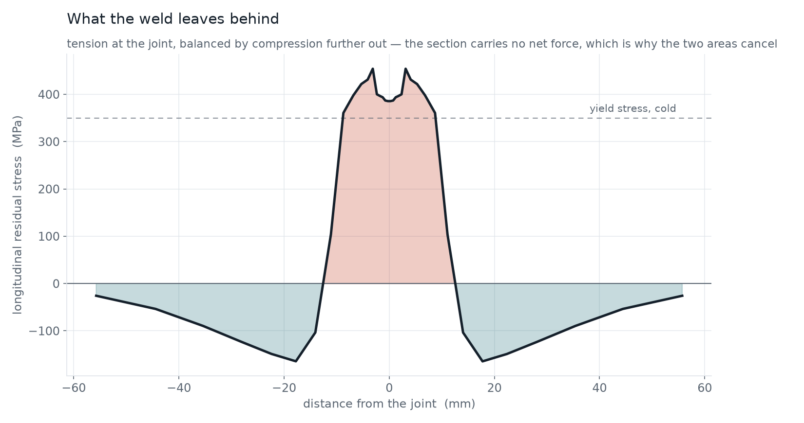
Longitudinal residual stress across the joint, tension at the weld and compression outboard — Longitudinal residual stress across the joint after twenty minutes of cooling. A tension plateau sits over the weld and its heat-affected zone, peaking at 454 MPa in the heat-affected zone just outside the fusion line — while the weld centerline itself, annealed as it resolidified, holds the **+386 MPa** quoted above — then drops through zero at about 13 mm from the seam into a broad compressive trough reaching −165 MPa. The two shaded areas very nearly cancel: the section carries no net force, because nothing external is pulling on it.

The tension at the weld line exceeds the room-temperature yield strength of the parent material, which sounds impossible until you remember the metal work-hardened on the way there. That is not a modeling artifact; welds routinely measure at or above yield along the seam, and it is the reason post-weld heat treatment and peening exist. It is also why a weld toe is such an unforgiving place to put a fatigue-critical detail: the mean stress there is already at the top of the material's range before the structure has been loaded at all.

The self-cancelling shape of the curve is a check in its own right. Integrated across the section the profile comes to a mean of 3.8 MPa against peaks of several hundred — the equilibrium a free plate must satisfy, arrived at by the solver rather than imposed.

The part that moves, and the part that stays put

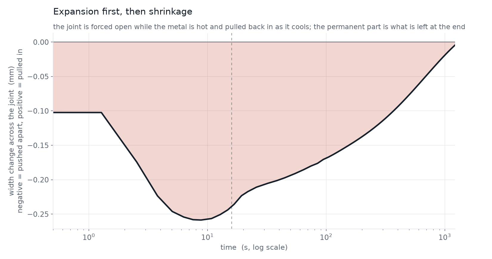
Width change across the joint through the arc and the cooldown — The joint's width through the whole cycle, on a logarithmic time axis. While the arc is on, the heated band forces the plate open by more than two tenths of a millimeter. Everything after that is contraction, most of it in the first two minutes, continuing for the full twenty. The permanent part is what is left at the far right.

Out-of-plane distortion comes to 0.12 degrees, with the seam standing 0.13 mm proud of the plate. That is a small angle, and it is small for a reason worth stating: this weld penetrates fully, so the whole thickness melts and contracts more or less together. Angular distortion is driven by the top of a joint shrinking more than its root, and a full-penetration single pass gives that asymmetry very little to work with. A partial-penetration weld, or a multi-pass one filling a V-groove from the bottom up, would bend the plate considerably more.

Transverse shrinkage is the honest disappointment. Measured across a 40 mm gauge either side of the seam the plates are drawn together by 0.053 mm; measured edge to edge across the full 124 mm plate the movement is essentially nil. Real butt welds shrink transversely by something closer to a millimeter, and the difference is the model's construction, not its arithmetic. There is no groove here to close and no filler metal being added — the bead occupies its final volume from the start and merely changes state. Most of the transverse shrinkage a fabricator measures comes from a gap being filled and a deposit solidifying into it, and that mechanism is simply absent. The plate is also free to move, restrained at three points only, so contraction that a clamped joint would convert into stress is instead absorbed as internal redistribution.

What a model like this is for

The seam takes sixteen seconds to lay down. The stress field that decides how the joint behaves for the rest of its life takes twenty minutes to develop, and by then there is nothing to see. That is the case for simulating welds at all: the information you want is invisible in the finished part, and expensive to get at afterwards by neutron diffraction or hole drilling.

What makes such a model worth acting on is not the sophistication of the physics but whether it can prove its own claims. This one is asked three questions before any result is quoted: does the heat source actually travel, does the energy balance close, and does the residual stress field carry no net force. Each has a number attached and each is checked on every run — because the failure mode that matters is not a model that crashes, it is a model that runs beautifully and is quietly answering a different question than the one you asked.

Revisions

v2 · Internal reviewReconciled the 454 MPa heat-affected-zone peak with the +386 MPa weld-centerline stress, stated the 20 C initial temperature, and re-attributed faster-than-Rosenthal cooling to surface losses.

Honest scope. The bead and the parent plates share nodes: this is quiet-element deposition, in which the bead's stiffness is switched on as it melts, rather than two physically separate plates being fused across a gap. It captures the joint being made in the sense that the bead carries no load until the arc reaches it, but it is not a model of gap closure, and the transverse shrinkage above is understated for exactly that reason. There is no filler-metal volume added and no groove. Above the liquidus the thermal conductivity is multiplied by five to stand in for the convective stirring of a real weld pool, which no pure-conduction model contains; without that stand-in the arc center climbs to temperatures no one should quote, and even with it the peak element temperature is not a quotable output — there is no vaporisation cut-off. The fusion and heat-affected zone extents are the trustworthy thermal results. Material properties are a generic mild steel with temperature-dependent modulus, yield, expansion, conductivity and specific heat, and latent heat smeared across a 50 degree melting range; they are not a specific certified grade. Convection is a uniform 15 W/m²K with radiation neglected, which makes the late cooldown slower than a real bench would be. Arc efficiency is folded into the 3 kW delivered figure rather than modeled. Residual stress is sampled on one element layer at mid-thickness, not integrated through the section. Single pass, no preheat, no filler chemistry, no phase-transformation plasticity — the last of which measurably changes residual stress in higher-carbon steels. Nothing here has been welded or measured on a bench.

Have a welded assembly that has to come out of the fixture within tolerance — and you need to know what the joint will pull before you cut metal? The same Ansys workflow behind this seam — LS-DYNA solving the thermal and mechanical problem together, a Goldak source tracked along a real path, quiet-element deposition so the bead only carries load once it has melted, and every run gated on whether the arc moved, whether the energy balanced and whether the residual field carries no net force — is how Rand Simulation helps fabrication teams find distortion and residual stress on screen instead of on the shop floor. That's innovation through insight.