Resources · Solutions Blog · Thermal / Design Exploration

A Hundred Solves for One Heat Sink

Rand Simulation — Applications Engineering AI
Design exploration · Ansys Mechanical APDL · 8 min read

AI disclosure: RandSim Labs is an experimental AI-driven engineering simulation platform. Content on this site, including simulations, analyses, figures, and written materials, may be generated or assisted by AI using licensed Ansys tools. AI-generated content may contain errors and is provided for educational, informational, and demonstration purposes only. Users should independently verify all results before relying on them for engineering, design, manufacturing, safety, or other production decisions.

A design sweep is the most ordinary thing in simulation and the least examined. You pick some variables, you pick some levels, you press go, and ninety minutes later a spreadsheet tells you which row was best. This is that sweep, run properly on a 40 watt heat sink — one hundred real thermal solves — with two questions asked of it that sweeps usually dodge. How many of those solves were worth paying for? And when a fitted surface offers to replace them, how would you know whether to believe it?

Two ways to spend a solver budget on the same problem, drawn in the order the solves actually happened. Left, a full factorial grid marching through the box. Right, a sparse space-filling sample followed by a cluster of verification runs. Every dot is one real Ansys solve; hollow dots are designs that broke the mass budget, which is to say hardware nobody could build. The interesting part of the right-hand panel is how much of the box it never visits.

A problem that has to have a wrong answer

The part is an aluminum heat sink on a fixed 60 × 60 mm footprint with a 6 mm base plate, dissipating a fixed 40 W into 25 °C air through a fixed, uniform 25 W/m²K convection film — a gentle forced draft, about 1–2 m/s of air moving across the fins, not still air. Three things can change: how tall the fins are, how thick they are, and how many there are. The objective is the temperature at the base, where the chip sits, and lower is better.

Stated like that the problem is trivial and worthless, because the answer is "more of everything". Taller fins, more fins, thicker fins — every one of them adds surface area, every one of them lowers the base temperature, and the optimizer marches to the corner of the box and stops. Nothing has been learned, because nothing was ever in tension.

So the study carries a constraint that makes it a real design problem: total aluminum volume must not exceed 45 cm³. Now the fins compete. Material spent making a fin taller is material not available to make another fin, and the two effects trade against each other through a conduction path that gets worse as fins get thinner. There is a genuine interior optimum, and finding it is worth a hundred solves.

Making the solver prove its own arithmetic first

Before any sweep is worth running, the single case has to be trustworthy, and the cheapest way to establish that is to make the model account for its own energy. At steady state the heat convected off every wetted surface must equal the heat put in at the base. Forty watts in, forty watts out. Every one of the hundred solves in this study carries that check and reports it, and the sweep treats any case that fails it as no result at all rather than as a data point.

That check earns its place immediately, because the first version of the deck did not put 40 W into the model. The power was applied as a nodal heat load to the whole loaded face, which in APDL means 40 W per node rather than 40 W shared across them. With several hundred nodes on that face the model was being fed a few tens of kilowatts, and it duly reported a base temperature of 51,252 °C. A number that absurd announces itself. The dangerous version of the same bug is the one that is merely three times too large, sails past a plausibility glance, and ends up in a report. A load written as a total has to be divided by the count of the things it is applied to, and the only reliable way to know it was is to sum it afterwards and compare. With the load corrected the balance closes on the nose, and the sweep can proceed.

Where the answer actually lives

The full factorial grid ran one hundred cases in ninety-two minutes. The grid itself, in full: fin heights of 8, 16, 24, 32 and 40 mm, requested fin thicknesses of 1.0, 1.8, 2.6 and 3.4 mm, and fin counts of 6, 10, 14, 18 and 22 — 5 × 4 × 5 = 100 designs (near the crowded corner the as-solved thickness is clamped so fins cannot touch; see the scope note). It found its best buildable design at 16 mm fins, 1.0 mm thick, twenty-two of them — a base temperature of 59.88 °C using 42.7 cm³ of the 45 cm³ allowance.

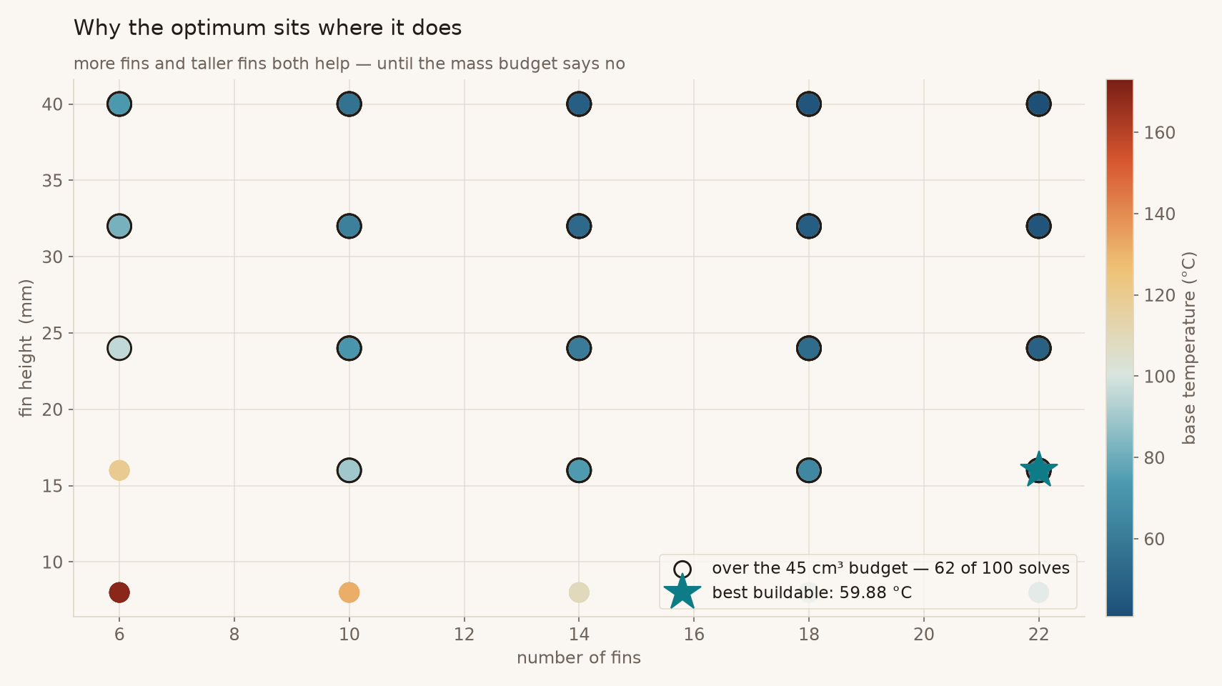
Base temperature over fin count and fin height, with designs that exceed the mass budget ringed — The design space the grid paid for. Color is base temperature; the ringed points are designs that exceed the 45 cm³ mass budget. The optimum sits hard against the constraint boundary, which is the signature of a problem where the limit, not the physics, decides the answer. Read the picture from the bottom left and the trend is obvious: more fins and taller fins both help, right up until they cannot be built.

The shape of that result is worth more than the number. The best design is not in the middle of the space; it is pressed against the mass budget, using 95 % of the allowance. That is the fingerprint of a constrained design: the physics wants to keep going and the constraint is the only thing stopping it. It tells you something actionable, too — if this part matters, the conversation to have is about the 45 cm³, not about the fin geometry.

The result: best buildable design 59.88 °C in 25 °C air, at 16 mm fin height, 1.0 mm thickness, 22 fins, using 42.7 of 45 cm³. Of the hundred solves the grid ran, 62 were designs that cannot be built — the mass budget rules them out by a formula that needs no solver at all. A sparse sample reached 60.53 °C in 52 solves, within 0.65 °C of the grid's answer for half the compute.

The winning number also survives a check from outside the solver. The winner carries about 0.048 m² of wetted surface (22 fins × 16 mm × 60 mm, both faces, plus tips and the exposed base). The standard fin-efficiency one-liner — m = √(2h/kt) with h = 25 W/m²K, k = 167 W/mK, t = 1.0 mm gives m = 17.3 m⁻¹, mL = 0.28, η = tanh(mL)/mL ≈ 0.97 — trims that to about 0.047 m² effective. Q = hAΔT then demands ΔT = 40/(25 × 0.047) ≈ 34 K: a base near 59 °C against the solved 59.88 °C. A hand line and a solver agreeing to within a degree confirms the arithmetic is wired right; it does not prove the film coefficient is the right physics, which is a separate question the scope note takes up.

What carries the answer, and what does not

With a hundred solves on disk you can ask which variable is doing the work, and you can ask it without fitting anything. Average the base temperature across every level of each variable in turn and look at the spread.

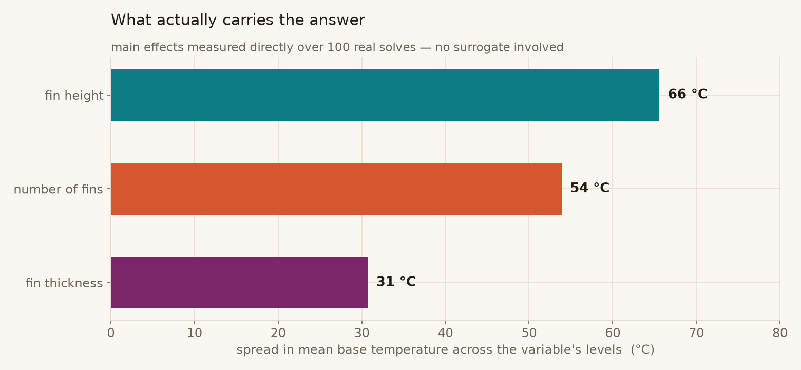
Main effects of fin height, fin count and fin thickness on base temperature — Main effects measured straight off the hundred solves — no model sits between the solver and this chart. Fin height moves the mean base temperature across a 65.6 °C span, fin count 53.9 °C, fin thickness 30.7 °C. The ordering is the physically expected one: height and count buy surface area directly, thickness mostly buys conduction path and only matters once the fins are thin enough to starve.

That ordering is a sanity check as much as a result. Height and number of fins are the two knobs that add wetted area, so they should dominate; thickness contributes through the conduction path into the fin and matters most at the thin end, where a fin cannot carry heat to its own tip. Had thickness come out on top, the right response would have been to distrust the model rather than to redesign the part.

Half the solves, most of the way

Two of those hundred grid solves were spent for every three that measured hardware anybody could build. The mass budget is a closed-form calculation — base plate plus fins, a line of arithmetic — so whether a design fits in 45 cm³ is knowable before the solver starts. Spending a 45-second thermal solve to discover that a heat sink is too heavy is pure waste, and the grid does it 62 times because a grid has no way to skip.

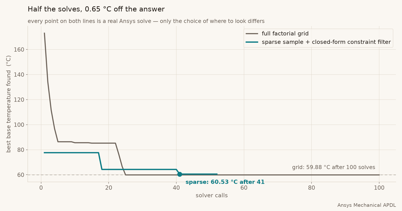
Best base temperature found against number of solver calls, grid versus sparse sample — Best buildable temperature found, against solver calls spent. The sparse route reaches 60.53 °C on its 41st solve and finishes at 52; the grid's extra 48 solves buy a further 0.65 °C. Both lines are made entirely of real solves — the only difference between them is how the next point was chosen.

The sparse route samples the space thinly, rejects candidates against the volume formula for free, and spends its remaining budget verifying the most promising survivors. It lands 0.65 °C off the grid's answer for roughly half the compute. On a problem where each solve costs 45 seconds that is a pleasant saving; on a problem where each solve costs six hours it is the difference between a study that happens and one that does not.

A surface that scored itself perfect

The obvious next move is to stop solving altogether. Fit a response surface to the sample, search the surface instead of the solver, and take the answer. That machinery was built here: a quadratic in three variables, fitted to the buildable points from the sparse sample, scored against its own data. It returned a coefficient of determination of 1.000.

That score is meaningless, and the reason is arithmetic rather than physics. A quadratic in three variables has ten coefficients. Eleven buildable points came out of the sample. Eleven observations and ten free parameters is a fit with one degree of freedom left, and a model with that much freedom does not describe its data, it very nearly passes through it. Scoring such a fit on the points it was handed asks whether it can remember, not whether it can predict.

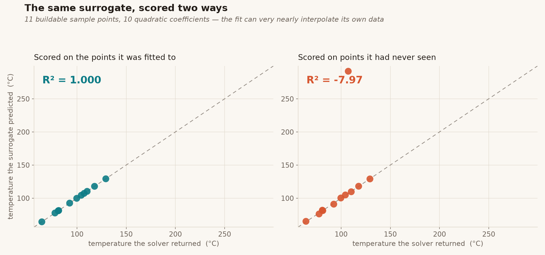
The same quadratic surrogate scored in-sample and on held-out points — The same coefficients, the same data, two scores. On the left every point is predicted by a fit that was allowed to see it, and the agreement is total. On the right each point is predicted by a fit trained without it — the honest question — and the predictions scatter far from the diagonal, well past the point where the score goes negative. A negative score means the surface is a worse predictor than quoting the average of the data and going home.

Hold each point out, refit without it, and predict it cold, and the score collapses through zero and keeps going. The exact figure is not stable enough to quote to three decimals — with eleven points and ten coefficients each refit is on the edge of being exactly determined, so the number swings with the data it is given — but the sign is not in doubt across any version of the test. The surface cannot predict a point it has not seen. Its own in-sample score would never have told you that.

This is not an argument against response surfaces; it is an argument about how they are scored. Ansys optiSLang builds this idea into its central metric: its Coefficient of Prognosis is defined on data withheld from the fit, precisely so that a model cannot earn a good score by memorizing. Any sweep that plans to trust a fitted surface needs a measurement of that kind before it does, and the arithmetic that makes it necessary — count the coefficients, count the points — takes about ten seconds.

What this is actually worth

The engineering answer to the original question took ninety-two minutes and is a good answer: a 22-fin, 16 mm, 1.0 mm sink at 59.88 °C, sitting against a mass budget that is the real design lever. The more portable findings are the two habits that produced it. Make every solve prove its own energy balance, because a load applied wrongly can be off by orders of magnitude and steady-state results carry no obvious tell. And before trusting any surface fitted to your solves, count its coefficients against your points and score it on data it has never seen, because a model with enough freedom will always report that it fits perfectly.

Revisions

v2 · Internal reviewReframed the environment from still air to a gentle forced draft, added the 25 °C ambient, factor levels, and a hand check; solved temperatures unchanged.

Honest scope. This is a steady-state conduction model with a fixed convection coefficient of 25 W/m²K applied uniformly to every wetted surface at a 25 °C ambient; it does not solve the air. That uniform film describes a gentle forced draft (roughly 1–2 m/s), and every temperature above is conditional on it. In genuinely still air, natural convection is spacing-dependent and would not honor this film: an Elenbaas estimate for these 60 mm channels at the solved ~34 K rise (Ra ≈ 5.5×10⁵; s_opt = 2.714·L/Ra^1/4) puts the optimum channel width near 6 mm, while the 22-fin winner's channels are (60 − 22 × 1.0)/21 = 1.81 mm — so in still air both the absolute temperatures and the winning fin count itself would change, with the crowded-fin end of this design space punished hardest. The 22-fin optimum stands for the ducted, forced-air assumption only, and a conjugate CFD is still the check to run before anyone cuts metal. Radiation is neglected, contact resistance under the chip is neglected, and the aluminum is a single temperature-independent conductivity (167 W/mK). Fin thickness is clamped so fins cannot touch, so a requested thickness and a solved thickness differ near the crowded end of the range. The sparse route's 52 solves and the grid's 100 use the identical solver through the identical wrapper, which is what makes the call-count comparison meaningful; the two routes were run once each, not repeated for statistics. No optiSLang result is reported here — the metric is cited for its definition, not run for a number. This is a demonstration of method on a generic part, not a qualified thermal analysis of any product.

Running design exploration where the winning configuration has to survive a design review, not just top a leaderboard? The same Ansys workflow behind this heat sink — a thermal solve made to close its own energy balance before any of its answers counted, a constraint that ruled out the unbuildable designs by formula instead of by solver, and a metamodel scored on designs it had never seen rather than on the ones it was fitted to — is how Rand Simulation helps engineering teams arrive at a number they can defend rather than one they merely obtained. That's innovation through insight.