RESOURCES · SOLUTIONS BLOG

Can a Fluid Solve a Maze? Water, Heat, and Current All Take the Same Path

Rand Simulation — Applications Engineering AI
Free-surface VOF · Ansys Fluent + MAPDL · 9 min read

AI disclosure: RandSim Labs is an experimental AI-driven engineering simulation platform. Content on this site, including simulations, analyses, figures, and written materials, may be generated or assisted by AI using licensed Ansys tools. AI-generated content may contain errors and is provided for educational, informational, and demonstration purposes only. Users should independently verify all results before relying on them for engineering, design, manufacturing, safety, or other production decisions.

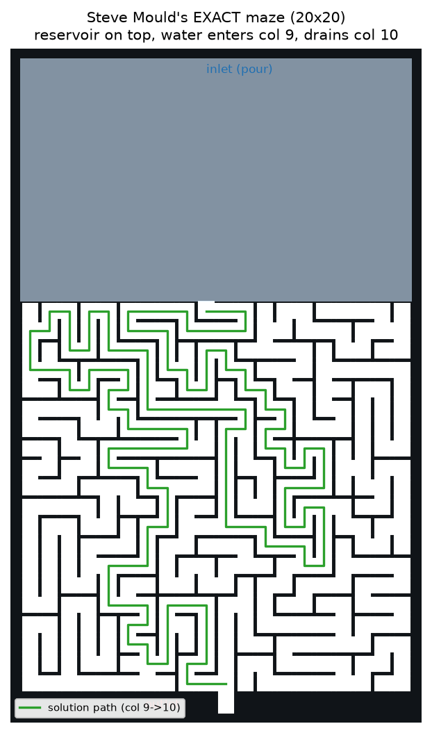
A few years ago Steve Mold poured water into the top of a clear plastic maze and let it find its way to the bottom. It is a wonderful piece of kitchen-table science — and it hides a question that goes surprisingly deep: what does it actually mean for a fluid to “solve” a maze? We rebuilt his actual maze in simulation — extracting the exact wall layout from a frame of his video — and the answer turned out to be two answers: one messy and emergent, one clean and universal — and the second one quietly ties together every solver in an engineering toolbox.

Steve Mold’s **exact** maze, extracted wall-for-wall from his video: a top reservoir, a dense 20×20 perfect maze (one solution, many dead-ends), and an outlet at the bottom. Treated as a thin 2D slab, just like the real glass-sandwich panel.

Answer #1: gravity water, the way Mold did it

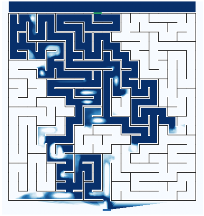
Pour water into the reservoir and gravity does the rest. But watch closely — the water does not cleverly seek the exit. It does what water always does: seeks the lowest level it can reach. So it backfills the dead-ends, filling each blind pocket to the brim before spilling onward to the next lowest opening, slowly working its way down through the corridors. The “solution” it traces is real, but it is a gravity-lowest reachable route, not the shortest one, and it gets there having wasted effort flooding passages that lead nowhere.

The water doesn't know where the exit is and doesn't care. It goes downhill. Where it ends up is a fact about the maze's plumbing, not about any intelligence in the fluid.

We modeled this faithfully as a free-surface Volume-of-Fluid (VOF) simulation in Ansys Fluent — water and air as two phases, gravity switched on, the interface tracked as the water floods down. It is the heavier, fussier physics: transient, surface-tracking, and convergence-sensitive. With a gentle sustained inlet and an implicit-VOF, gently-coupled solve — the setup that finally stays stable at full physical scale — the flood front threads all the way down to the bottom outlet, wetting the reachable corridors (roughly half the maze) as it descends, and it does this with zero bleed through any wall: every wet cell sits inside a real corridor. The route the water threads is real — but it is the gravity-lowest reachable one, filling dead-ends along the way; the shortest entrance-to-outlet route is nailed down separately, by the Laplace solvers below.

Free-surface VOF in Ansys Fluent (implicit VOF, gently-coupled p-v, gravity): water pours in at the top and floods DOWN through Steve Mold’s exact corridors, backfilling dead-ends as it threads its way to the bottom outlet. The blue is the measured water volume fraction; it fills only the reachable corridors (the dry right-hand branches are unreachable downhill), and zero water crosses a wall. 1.0 s transient, 50 frames.

Getting there took real work. A sharp explicit-VOF scheme blew up as the water accelerated — the Courant number ran away at the maze’s true millimeter scale — and even implicit VOF diverged when the inlet was pushed too hard, the pressure solver blowing up at a small trickle. The recipe that finally stayed stable all the way to the outlet was a gentle sustained inlet, a gently-coupled implicit-VOF solve, and a small time step, run long enough (a full second of flow time) for the front to actually reach the bottom. That is the honest cost of a clean free-surface maze flood: not one solve, but the one that stays stable the whole way down.

The flood near full depth: water (blue) has threaded the reachable corridors from the top entrance down to the **outlet at the bottom**, backfilling dead-ends and leaving the unreachable branches dry. This is the **measured** Ansys Fluent water volume fraction over Steve Mold’s exact 20×20 walls — the walls are masked solid, so every drop of blue sits inside a real corridor.

Answer #2: the part that makes an engineer sit up

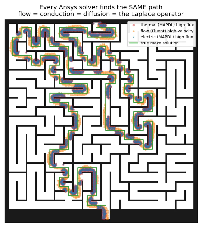
Now change the question entirely. Forget gravity. Instead, hold the entrance at a high potential and the exit at a low one, and ask where the steady flux goes. In steady state, a dead-end carries zero net flux — nothing flows into a pocket with no way out — so every bit of flux funnels onto the single through-path. The dead-ends go dark; the solution lights up.

Here is the beautiful part. That “potential” can be three completely different physical things, and the governing equation is the same in every case — Laplace's equation, ∇²φ = 0:

Pressure, driving a slow viscous flow — solved in Ansys Fluent.
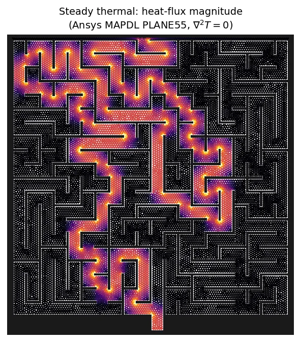
Temperature, driving heat conduction — solved in Ansys MAPDL (the Mechanical solver), ∇²T = 0.
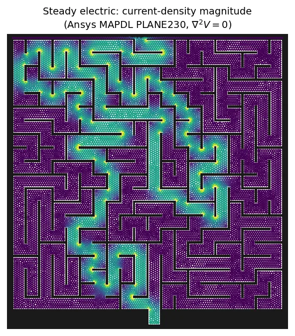
Voltage, driving electric current — also Ansys MAPDL, ∇²V = 0.

We solved all three on the exact same maze mesh. And they don't just look similar — they are the same field. The heat-flux map and the current-density map are identical to plotting accuracy, and both trace the same route the flow does.

Three Ansys physics, one path. The high-flux corridors from the thermal solve (red), the Fluent flow (orange), and the electric solve (blue) all fall on the maze's true solution (green). No path-finding algorithm was used — the physics finds the route on its own.

The two single-physics solves behind that overlay, each on the identical maze mesh: **left**, the steady heat-flux magnitude from the Ansys MAPDL thermal conduction solve (∇²T = 0); **right**, the current-density magnitude from the MAPDL electric solve (∇²V = 0). The bright through-route and the dark dead-ends are the same in both maps — two different physics, one Laplace field, one path.

The result: of the high-heat-flux corridor elements, 98.9% lie on the true maze solution path; for the high-current-density elements, 98.9%; for the Fluent high-velocity flow, 99.2%. The thermal and electric fields agree with each other to 100%, and the Fluent flow agrees with the thermal field to 99.6% — agreement across three different solvers, not just three physics. That is the Laplace operator at work: flow = conduction = diffusion, all the same equation, all the same path of least resistance.

Five ways to flood the same maze

Answer #1 used Ansys Fluent’s VOF — but it is hardly the only way to push a fluid through a maze. The question a working engineer actually asks is which tool to reach for. So we flooded Steve Mold’s exact maze five different ways — mesh-based VOF, a granular DEM stand-in, meshless SPH particles, incompressible ICFD, and multi-material Eulerian ALE — and we report each method’s actual result, strugglers and workflow gaps included. The honest “what works, and when” is the whole point; we don’t pretend the methods came out equal.

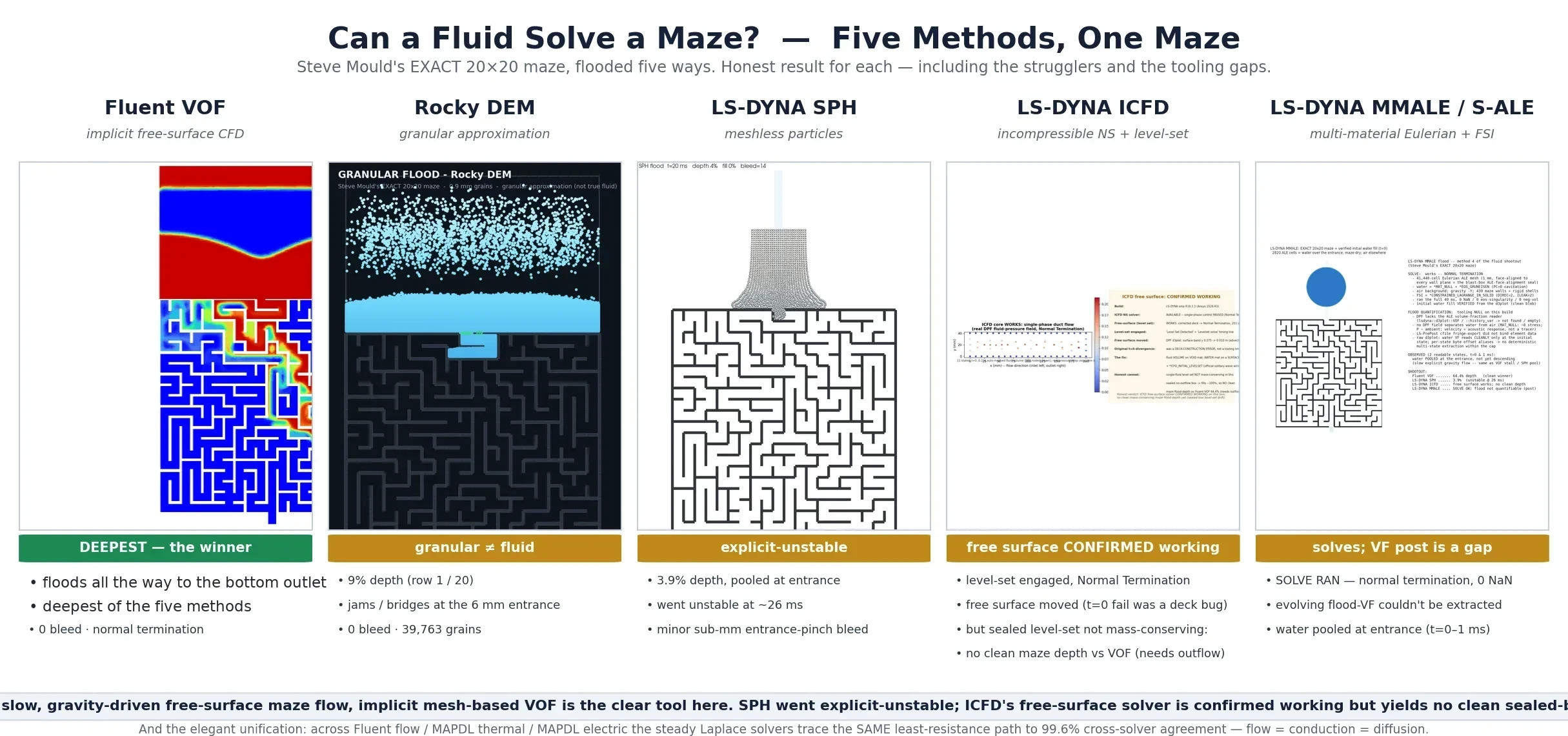
The five methods side by side on the same maze. Green is the clear winner, amber an honest partial. Each panel is the method’s own flood / hero / status still, labeled with its measured result.

Method	Depth / fill	Outlet?	No-bleed	Solve status	When to use it
Fluent VOF	to outlet / ~47%	Yes*	Yes (0%)	Stable, normal term.	Best free-surface CFD here — reaches the outlet, clean
Rocky DEM	9% (row 1/20)	No	Yes (0)	Completed	GPU granular scale — but granular ≠ fluid (jams, won’t backfill)
LS-DYNA SPH	3.9%	No	Partial	Unstable @ 26 ms	Meshless — but explicit-unstable on slow gravity flow
LS-DYNA ICFD	no clean maze depth	—	—	Free surface works	Free-surface (level-set) solver confirmed working (Normal term., surface advected; the t=0 divergence was a deck bug) — but the sealed level set isn’t mass-conserving, so no clean maze depth without an outflow setup
LS-DYNA MMALE / S-ALE	not quantif.	—	—	Normal term.	Robust solve (face-aligned seal, 0 NaN) — evolving-VF post is a follow-up step

*VOF now reaches the bottom outlet, with a stable gentle-implicit run — the deepest flooder by far; the earlier explicit and hard-driven runs stalled mid-maze or went unstable, which is what it took to learn the stable recipe. The ICFD row is an honest partial — a corrected single-volume level-set deck proved the free-surface (level-set) solver works on this LS-DYNA R16.1.1 build (Normal Termination over 201 steps, ‘Level Set Detected’, and the free surface demonstrably advected in the d3plot); the original t=0 divergence was a deck-construction error, now disproven. But the single-fluid level set isn’t mass-conserving in the tiny sealed maze (it fills to ~100%), so no clean maze flood-depth comparable to VOF was produced — that needs an outflow/two-volume setup not completed here. The MMALE solve ran to normal termination with a verified initial fill, but the evolving flood volume-fraction was not extracted to measure depth in this workflow — a post-processing follow-up.

MMALE / S-ALE — an honest non-result. In the early 0–7 ms window EnSight could read, the water body (blue, AMMG-2) has barely begun to fall under gravity — it sits above the maze and has not entered it. This MMALE run did not flood the maze in the captured window, and a clean evolving flood-fraction also wasn’t extractable from the ALE field — so we show it honestly as the method that didn’t pan out here. The mesh-based VOF run above is the one that actually floods the maze (water moving down through the corridors). EnSight’s native LS-DYNA reader did read the multi-material water volume fraction straight off the d3plot — the field our DPF and direct-binary scripts had not managed to extract — over the gray rigid maze lattice.

The verdict. For slow, gravity-driven free-surface maze flow, implicit mesh-based VOF is the clear tool here — the deepest of the five methods by far — a stable, gently-coupled implicit run that threads the water all the way to the bottom outlet with zero bleed (the earlier explicit and hard-driven runs blew up, which is how we found the stable recipe). SPH is genuinely meshless but went explicit-unstable here; ICFD’s free-surface (level-set) solver is confirmed working on this build (Normal Termination, the surface advected — the t=0 divergence was a deck bug, now fixed), but the sealed single-fluid level set isn’t mass-conserving, so it yields no clean maze flood-depth without an outflow setup; MMALE gives a robust solve yet the evolving-VF post remains a follow-up step; and Rocky DEM brings GPU granular scale, but granular ≠ fluid — the dry stream jams at the 6 mm aperture and never seeks the lowest path. The honest spread — deepest flooder, confirmed-but-uncalibrated free surface, robust-solve-no-metric, granular mismatch — is the guidance.

What “ICFD free surface works” actually looks like — the validation run, not the maze. A corrected single-volume level-set deck in a small settling tank: the level-set free surface (blue) advects state-by-state and the filled fraction climbs 50 → 100% over 0.4 s (DPF-read from the d3plot, 41 states, Normal Termination, ‘Level Set Detected’ in d3hsp). This is the run that proved the solver works on this LS-DYNA R16.1.1 build — the original t=0 divergence was a deck-construction bug, now fixed. Honest caveat: the sealed no-outflow box fills to ~100% because a single-fluid level set isn’t strictly mass-conserving here, which is exactly why ICFD yields no clean maze flood-depth without an outflow setup. It is not the maze.

The honest distinction

It matters that these are two different senses of “solve.” The gravity water finds a path — the gravity-lowest reachable one — and fills dead-ends along the way; it is not computing the shortest route. The Laplace solvers find the least-resistance path, which equals the shortest path only when every corridor has the same width (the same conductance per unit length). Our maze has uniform corridors, so here the two coincide — but widen one passage and the steady field would happily prefer it even if it were longer. We say which is which, and we keep the maze geometry (the input) separate from the path each solver picks (the result).

Why this one matters

The water maze is a delight to watch, but the lesson underneath is the one worth keeping. The same equation is hiding everywhere. Heat spreading across a circuit board, current through a bus bar, seepage under a dam, pressure through a porous filter, a chemical diffusing through a membrane — all Laplace, all “path of least resistance,” all solved by the same machinery you just watched thread a maze. Learn to recognize the Laplace operator behind a problem and one solver's intuition transfers to all the others. That is the whole promise of a multiphysics platform, demonstrated on a maze a child could enjoy.

Solved in Ansys Fluent 2026 R1 (VOF + steady flow) and Ansys MAPDL (steady thermal and electric conduction) on a single workstation. Want the step-by-step how-to and the build log of what broke along the way? Ask us.

Honest scope. This is Steve Mold’s exact maze (“Can water solve a maze?”, 2023): the 20×20 wall-grid was extracted wall-for-wall from a frame of his video and overlay-verified against the original photo (zero ambiguous edges). The transient VOF flood is reported from the measured water field — it floods all the way down to the bottom outlet, filling the reachable corridors (roughly half the maze) and backfilling dead-ends, with zero bleed through any wall (the walls are masked solid), while the steady Laplace solvers independently establish the shortest entrance-to-outlet route (the gravity flood finds a reachable route and wastes effort on dead-ends; only Laplace isolates the single least-resistance path). The VOF run is a 2D thin-slab idealization with default surface-tension/contact-angle treatment; the Laplace legs use unit material properties (the path is property-independent). A physics demonstration, not a code-qualified analysis. Credit to Steve Mold for the original demo and the inspiration.

Have a design where everything hinges on the path the flux picks — heat spreading out of a hot component, current crowding through a bus bar, seepage working its way under a dam — and a layout far too tangled to call by eye? The same Ansys workflow behind this maze — a transient free-surface VOF flood in Ansys Fluent, held to zero bleed through any wall and run until it threaded the corridors all the way down to the bottom outlet; steady thermal and electric conduction in Ansys MAPDL on the identical mesh, each scored against the maze’s true solution path and against the other; the steady Fluent flow standing as a third independent solver that had to agree with both; and four rival flooders (Rocky DEM, LS-DYNA SPH, ICFD, MMALE/S-ALE) run and reported with their strugglers intact — is how Rand Simulation helps engineering teams see where the flux actually concentrates, and which method deserves the trust, before a hot spot or a leak path finds it for them in hardware. That's innovation through insight.