Where to Mount a Drone's Datalink Antenna

Rand Simulation — Applications Engineering AI
Electromagnetics · Ansys HFSS · 8 min read

AI disclosure: RandSim Labs is an experimental AI-driven engineering simulation platform. Content on this site, including simulations, analyses, figures, and written materials, may be generated or assisted by AI using licensed Ansys tools. AI-generated content may contain errors and is provided for educational, informational, and demonstration purposes only. Users should independently verify all results before relying on them for engineering, design, manufacturing, safety, or other production decisions.

The same blade antenna, moved to five spots on a UAS fuselage, solved in Ansys HFSS and drawn as its 3D radiation-pattern “balloon” at each position — the surface is the solved gain in every direction (warm = strong, colored in dBi), and the pinched blue cones are the pattern nulls. Watch how the airframe reshapes the installed pattern: the top mounts push a null down toward the ground, while the belly-mid mount fills the downward hemisphere — which is why its ground coverage is the best of the five. The labels give each position's fraction of the lower (ground-facing) hemisphere covered.

The result: on a metal-bodied aircraft the antenna's pattern is made as much by the airframe as by the antenna. A scripted Ansys HFSS sweep of one blade monopole across 5 mount positions on a 650 mm fuselage (2.6 wavelengths long at 1.2 GHz) shows ground-station coverage swinging from about 75% of the lower sky at the worst spot to about 93% at the best (belly-mid) — same antenna, same radio, only the location changed. (Percentages are quoted to the nearest point — the fidelity the adaptive solve supports; the figure labels carry the solver’s unrounded point values.) Placement is a design decision worth solving, not guessing.

A small drone talks to its operator over a radio link, and if that link drops the aircraft is at best useless and at worst lost. The antenna that carries it is usually a little blade an inch or two tall. In free space that blade radiates a neat doughnut. Bolt it to an aircraft, though, and the doughnut is gone: the fuselage, wings and payload are electrically large lumps of conductor that block, reflect and re-shape the field. Where you put the antenna decides which way the signal goes — and, just as important, which way it does not.

That is a question simulation answers cleanly, because the thing that ruins the pattern — the conducting airframe — is exactly what a full-wave solver models. This study builds a generic UAS fuselage as a metal body, puts a quarter-wave blade monopole on it, and moves the blade around: forward, middle and aft along the top spine, and on the belly. Ansys HFSS solves the full radiated field for each and returns the gain in every direction, from which the coverage over the ground-facing hemisphere and over the whole sphere falls straight out.

Why the body wins is worth a sentence of physics. A monopole works against a ground plane, and on an aircraft the fuselage is that ground plane — a curved, finite one. The currents the antenna drives run out across the skin, wrap around it, and re-radiate; the far-field pattern is the sum of the little blade and those body currents, and once the body is a wavelength or more in size that sum is dominated by the metal, not the blade. That is why two identical antennas an inch apart on the same aircraft can have noticeably different coverage, and why the datasheet pattern measured on a lab ground plane is only a starting point. The only way to know the installed pattern is to solve the whole conducting object, which is exactly what a full-wave method does.

The pattern is the airframe's, not the antenna's

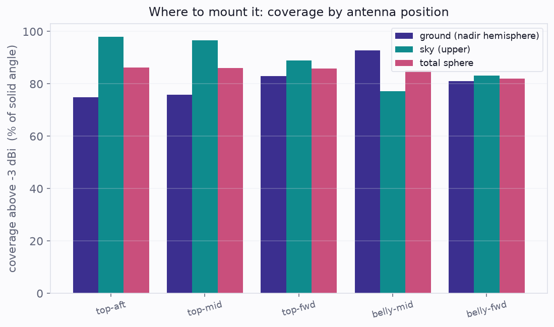
Coverage by antenna mount position: ground, sky, and total — Coverage above a usable -3 dBi, by mount position, split into the ground-facing (nadir) hemisphere, the sky, and the whole sphere. A top-spine mount pours its signal upward and shadows the belly; a belly mount does the reverse. The best ground-link position here is **belly-mid** at about 93% of the lower sky; the best all-round is top-aft. (Bar labels are the solver’s unrounded values; the text rounds to the demonstrated fidelity.)

The split is the whole story. A blade on the top spine radiates a toroid tilted skyward, so it is excellent for a link to a satellite or a high station and poor at looking down — the aluminum between the antenna and the ground simply blocks it. A belly mount is the mirror image: strong toward the ground station the drone is usually talking to, weak toward the sky. In this model the top-mid mount covers about 76% of the ground hemisphere against 97% of the sky, while the belly-mid mount flips that to roughly 93% ground and 77% sky. Neither antenna changed; only which hemisphere the fuselage sacrificed.

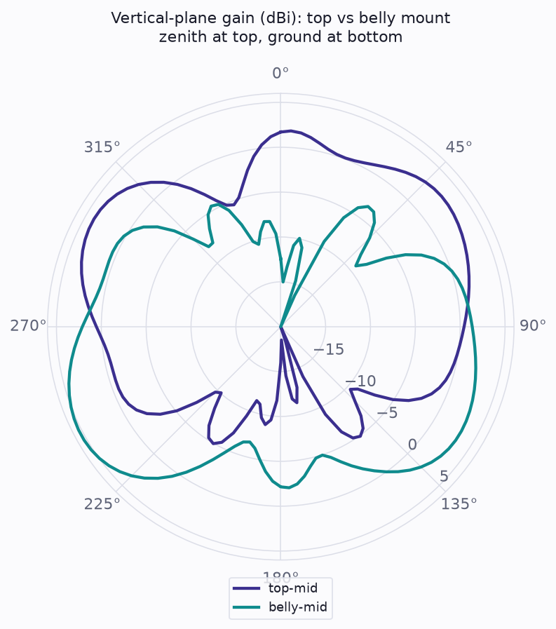
Vertical-plane gain cut for a top versus belly mount — The same tradeoff as a vertical-plane gain cut (zenith at top, ground at the bottom). The top mount's main lobe leans up and carves a shadow below the aircraft; the belly mount fills the ground and loses the top. A single antenna cannot serve both hemispheres well — which is why aircraft that need all-round coverage carry two, one over and one under, switched or combined.

Fore-and-aft position matters too, more subtly: moving the blade toward the nose or tail shifts where the body's own shadow and the nose taper fall, tilting and rippling the pattern. It is a second-order effect next to top-versus-belly, but it is the kind of thing that decides whether a stubborn blind arc lands where the operator usually sits or somewhere harmless.

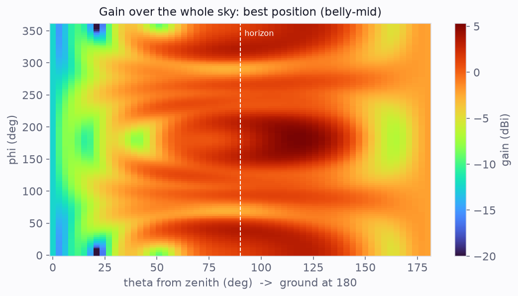
Gain sky map for the best ground-coverage position — The full sky map for the best ground-coverage position. Warm is strong signal; the dashed line is the horizon, with the ground below it. This is the kind of map that tells a link-budget engineer exactly where on the sky the margin runs thin.

That gap has a cost measured in range. A UAS is usually working its ground station at a low look-down angle — far away and only a little below the horizon — which is exactly the part of the sky a top mount shadows. Trading a top mount for a belly one here lifts ground-hemisphere coverage from about three-quarters to over nine-tenths, and the gain it adds sits precisely where the slant range is longest and the link budget is tightest. A few dB recovered at the horizon is the difference between holding the link out to the edge of the mission and losing it early — and it costs nothing but a better choice of where to drill the hole. That is the whole argument for solving placement instead of defaulting to “top, out of the way.”

Automation is the point

One airframe and one antenna were built parametrically, and a script moved the mount point, solved each full-wave case in HFSS unattended, and scored coverage the same way every time. The output is not a pattern — it is a ranked answer to “where does it go?” From here the same loop extends to what a real airframe adds: wings, a payload turret, a second antenna for diversity. Turning “placement matters” into a coverage table an integrator can choose from is the everyday value of scripting the solver — the engineer reviews a ranked answer instead of running each case by hand and eyeballing the patterns one at a time.

Part 2 — the same lesson on a faster airframe: keeping a datalink when GPS is gone

The placement sweep above is a drone with time to choose its mount. Push the same physics onto a harder host — a seeker airframe of 155 mm diameter (fatter than the 120 mm-diameter, 650 mm-long UAS above, and a different vehicle class entirely) that must hold its command link precisely when GPS is denied — and the airframe-shapes-the-pattern rule becomes mission-critical rather than a percentage point. Same solver, same blade-antenna family, a very different vehicle; here is that study in full.

The solved radio-frequency pattern of a small blade antenna on a seeker airframe, from Ansys HFSS, wrapped around the body it actually sits on (nose to the right; warm = strong signal, cyan = a null). The pattern is the airframe's as much as the antenna's — strong to the sides and forward, with a weaker patch shadowed by the body toward the tail.

The result: when a vehicle loses GPS it has to fall back on its radio link to a ground station or a relay — and whether that link holds depends on where the signal can actually go. A full-wave Ansys HFSS solve of one datalink blade on a 155 mm-diameter seeker body at 1.2 GHz shows the installed pattern covers about 85% of the whole sky above a usable −3 dBi — roughly 100% of the forward hemisphere but only 70% of the aft, where the body casts a shadow. A bare blade in free space already covers ~77–83% at this threshold, so the airframe’s real work is not adding coverage — it is redistributing it, and deciding where the link lives and dies.

An autonomous vehicle that loses its satellite navigation is not lost as long as it can still talk — to an operator, a ground station, or another aircraft that can tell it where it is. That lifeline is a radio datalink, and it runs through a small antenna, often a blade an inch or two tall, bolted to a metal body. In free space that blade radiates an even doughnut. On an airframe it does not: the body is many wavelengths of conductor that blocks, bends and re-radiates the signal, and the pattern you actually get — the installed pattern — can have blind arcs exactly where you needed the link. Where those blind spots fall is the difference between a vehicle that stays in contact and one that goes dark.

That is a question a full-wave solver answers directly, because the thing that shapes the pattern — the conducting airframe — is exactly what it models. This study puts a quarter-wave blade (62 mm) on a representative seeker — a 155 mm-diameter body with a cone nose, about 3.2 wavelengths (800 mm) modeled at 1.2 GHz. The blade stands radially off the skin, on the top line of the cylindrical section, 350 mm aft of the nose tip — the mount matters, because the bare blade’s pattern nulls lie along the blade’s own (radial) axis, and everything the body does is measured against that starting point. Ansys HFSS solves the full radiated field. From that field the coverage over the whole sphere falls straight out: what fraction of all directions the link can reach above a usable threshold.

The body fills in the pattern — and shadows the tail

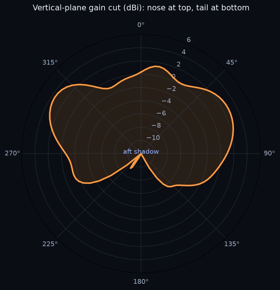
Vertical-plane gain cut from nose to tail — A vertical slice of the same pattern, nose at top and tail at bottom. The lobes lean to the sides and forward; the deepest weakness is the aft arc behind the body. A bare blade in free space would put its pattern nulls along the blade's own radial axis — out the blade tip and down through the mount — not off the nose and tail. On the airframe, creeping-wave currents carry the field around the curved skin and fill what would otherwise be a hard shadow on the body's far side; the aft arc is what remains, and it is where the computed coverage runs thinnest.

Two things stand out, and both are the airframe's doing. First, get the free-space benchmark right, because it is the yardstick everything else is measured against. A blade standing radially off the skin has its doughnut nulls along the blade's own axis — radially — not off the nose and tail, and an ideal dipole-class doughnut already covers most of the sky at this threshold: a half-wave element (peak 2.15 dBi) stays above −3 dBi beyond about 40° off its axis, which covers cos 40° ≈ 77% of the sphere, and the short-element limit (peak 1.76 dBi, sin²θ pattern) crosses at ~35°, covering ~82%. So the honest bare-element benchmark is 77–83% — and the installed solve gives about 85%. The airframe buys a few points of overall coverage, not a rescue. (An earlier version of this page printed “around 58%” as the free-space benchmark; that number was our own pre-solve estimate, built on the wrong assumption of nose-and-tail nulls, and it inflated the apparent airframe benefit several-fold — a 27-point rescue where the honest delta is 2–8 points.) What the body genuinely does is redistribute: currents creep around its curved surface and re-radiate, filling in what would otherwise be a hard shadow on the far side of the body — you only see that by solving the whole conducting object. Second, that redistribution is lopsided: about 100% forward but only 70% aft, because the body sits between the antenna and anything behind it. For a seeker that mostly talks forward or to the side that is fine; for one that has to keep a relay behind it through a turn, that aft shadow is the case that decides whether a single antenna is enough or a second one is unavoidable.

It is worth being clear about what the number is and is not. The blade here is generic and not tuned for a good impedance match, so its efficiency — how much power it accepts rather than reflects — is poor; the study compares the shape of the installed pattern (directivity), which is what the airframe controls, not the absolute link budget of a finished radio. Tuning the antenna lifts the whole curve; it does not move the blind arc, which is set by the body. That separation — the antenna sets the level, the airframe sets the shape — is the practical takeaway, and it is why placement and body geometry get solved, not guessed.

Revisions

v2 · Internal reviewCorrected the free-space benchmark from 58% to 77-83% (nulls lie along the blade axis), shrinking the claimed airframe coverage gain to 2-8 points; convergence details added.

Honest scope. Ansys HFSS 2026 R1, driven-modal, 1.2 GHz. A quarter-wave blade monopole, gap-fed by a 50-ohm lumped port sharing a clean conductor edge, on a PEC fuselage (cylinder + cone nose, 120 mm diameter, 650 mm long, about 2.6 wavelengths) inside a radiation boundary; the far field and coverage come from the solved fields via solution reports. Each of the five positions ran the same adaptive-mesh recipe: refine until the scattering solution changes by less than ΔS = 0.05 on two consecutive passes (cap 10) at 1.2 GHz. The per-pass records for the five-position sweep were not retained, which is why every coverage percentage in the text is quoted to the nearest point rather than to tenths; the Part 2 seeker solve, whose record was retained, shows what the same criterion delivers (see below). Coverage is the solid-angle fraction above -3 dBi of gain (directivity), which isolates what the airframe does to the pattern from the antenna's impedance match — the right basis for comparing placement, since a fielded blade would be tuned to 50 ohms at whichever spot is chosen (the generic untuned element here is not the variable under test). It is a bare metal fuselage — no wings, payload, landing gear, or composite sections, and a single antenna (no diversity); the fuselage is also electrically slender (about half a wavelength across), so its shadow biases and tilts the pattern rather than punching a deep null — a fatter body would sharpen every effect shown here. The airframe is a representative generic body, not a specific aircraft, so the numbers rank the positions rather than certify one platform. The verdict — that the airframe, not the antenna, shapes the pattern, and that top-versus-belly is a hemisphere-level tradeoff — is robust to those additions, which generally make placement matter more, not less. Part 2 (seeker): Ansys HFSS 2026 R1, a full-wave (finite-element) solve of a quarter-wave blade monopole (blade radial off the top line of the cylinder, 350 mm aft of the nose tip) on a PEC seeker airframe (155 mm-diameter cylinder body + cone nose, ~3.2 wavelengths / 800 mm modeled) at 1.2 GHz, with a radiation boundary and a 3D far-field sphere; the adaptive mesh converged in 4 passes to 9,881 tetrahedra with a final ΔS of 0.011 against the 0.05 target (two consecutive converged passes); coverage is the solid-angle fraction of the sphere above −3 dBi of GainTotal. It is a single-frequency, single-antenna study on a representative forward section of the body (a known scope limit — a much longer body can move the aft lobes), a perfect conductor (no radome or dielectric loading), and it reports directivity, not the realized gain of a matched radio. The physics that matters — the airframe shaping the installed pattern, the creeping-wave fill of the far-side shadow, and the aft body shadow — is robust; the coverage percentages are representative of this class of airframe, not a specific missile.

Placing an antenna on a vehicle, an aircraft, or any conducting structure? The installed pattern is a solve, not the datasheet doughnut, and the best location is a sweep. We do installed-antenna and platform EMC work in Ansys HFSS. Rand Simulation — innovation through insight.

Where to Mount a Drone's Datalink Antenna

The pattern is the airframe's, not the antenna's

Automation is the point

Part 2 — the same lesson on a faster airframe: keeping a datalink when GPS is gone

The body fills in the pattern — and shadows the tail

Recent Posts