Resources · Solutions Blog · Computational Fluid Dynamics / HVAC

Why a Heat-Recovery Core Doesn't Share Air Evenly

Rand Simulation — Applications Engineering AI
Heat transfer · Ansys Fluent · 9 min read

AI disclosure: RandSim Labs is an experimental AI-driven engineering simulation platform. Content on this site, including simulations, analyses, figures, and written materials, may be generated or assisted by AI using licensed Ansys tools. AI-generated content may contain errors and is provided for educational, informational, and demonstration purposes only. Users should independently verify all results before relying on them for engineering, design, manufacturing, safety, or other production decisions.

Sizing a heat-recovery core is one of the tidiest calculations in building services. Effectiveness-NTU is an exact solution of the idealized problem, it needs no solver, and for this core — 127 slots in a 298 mm stack, alternating supply and exhaust so 64 carry the supply air — it says that air leaves at 14.9 °C on a -5 °C day, an effectiveness of 0.766. It gets there by assuming every supply channel receives the same air. Nothing in the method checks that, and nothing in the method could.

What a heat-recovery core does, and what this study is really about. Warm stale air leaving the house crosses cold fresh air coming in, and the plates hand the warmth across between them — a schematic, with the stream temperatures set by the core's rating: it recovers 77 % of the 26-degree gap (an effectiveness of 0.766), so on a -5 °C day the fresh air arrives near 15 °C. The rating that promises this assumes every supply channel gets the same air. It does not, and that is what the CFD below is for.

The result: a side-entry header delivers a channel-flow spread of 25 % — the coefficient of variation (one standard deviation as a fraction of the mean), not the peak-to-peak range. The best-fed channel takes 145 % of its fair share and the most starved gets 76 %, across a stack whose slots are identical. That costs 0.82 points of effectiveness, 0.766 down to 0.758 — and a penalty curve written down before the solve predicted 0.757, within 0.0006 of it.

What the one-line method assumes

The core is a 298 mm stack of 2.0 mm slots between 300 mm square polymer plates, passing 250 m³/h. Supply and exhaust alternate — every plate needs one stream on each face or there is nothing to exchange across — so 64 slots carry the supply and each runs at Reynolds 501. That is laminar, which matters more than it sounds: in fully developed laminar flow the Nusselt number is a constant, so the heat-transfer coefficient stops depending on flow rate and depends only on the channel height. NTU 3.27, effectiveness 0.766, 1725 W recovered, 29 Pa across the core.

Two asterisks on that firmness, and they bracket everything that follows. The wall in a recuperator is neither isothermal nor constant-flux, and the two textbook Nusselt numbers that bracket it give 0.766 and 0.750. "Fully developed" is not quite true either: the thermal entry length is 71 mm of a 300 mm plate, about 24 % of it, over which the local Nusselt number is higher — so the real ideal sits a little above 0.766. Neither is resolved here, and both are worth keeping in view alongside the effect this study is about.

What none of that touches is the assumption underneath. Everything above is a statement about one channel, multiplied up, and asked to stand for 64.

The header does not cooperate

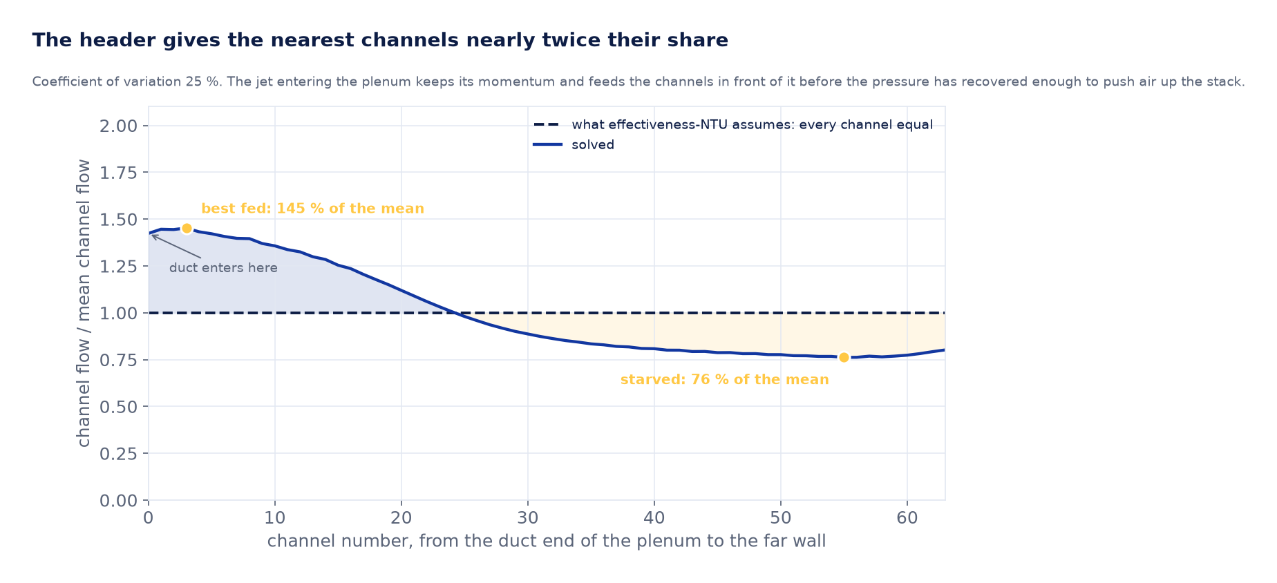
The solved velocity field in the inlet plenum and the first stretch of the core, with a reader walking down the stack one supply channel at a time. The field is a single steady solve; what moves is the eye, not the flow. The channels in front of the duct take about half again their share, and the middle of the stack goes short.

Flow per supply channel across the stack — Flow in each supply channel as a fraction of the mean, from the duct end of the plenum to the far wall. The dashed line is what effectiveness-NTU assumes. Nothing about the channels differs — they are identical slots between identical plates.

Air arrives in the plenum with momentum, and what each channel gets is set by the static pressure that reaches it. Two effects compete. The jet runs head-on into the channels directly in front of the duct and stagnates against them, converting dynamic head into static pressure and pushing hard into those slots. Meanwhile air that has to travel further up the plenum loses total pressure to friction and turning on the way. In this geometry the first effect wins: the near channels take 145 % of the average, the flow crosses its fair share around channel 24, and the far end settles near 76 %.

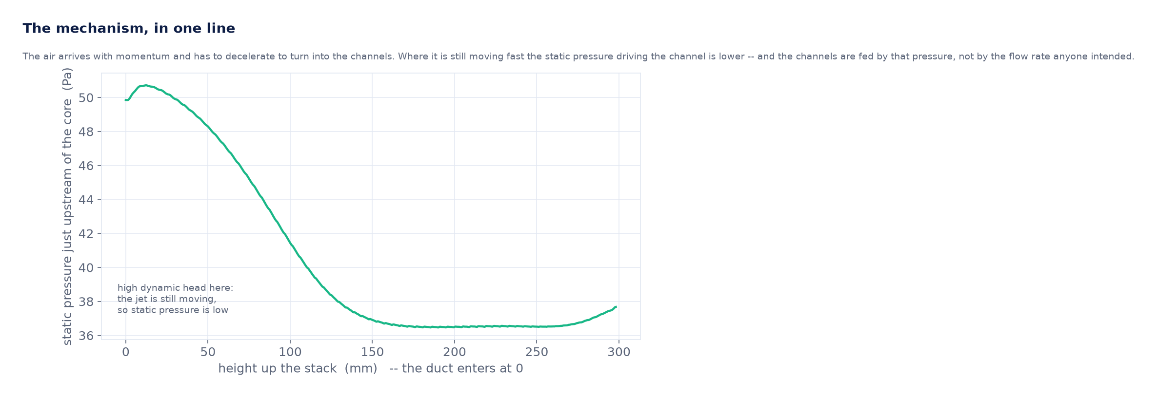
Static pressure along the plenum — Static pressure just upstream of the core face, up the stack. This is the driving pressure each channel actually sees.

The solved field makes it concrete: 50 Pa at the duct end, where the air has stagnated to a standstill against the channel mouths, falling to about 37 Pa across most of the rest of the stack. Total pressure falls monotonically along the plenum, 52 Pa to 38 Pa — so this is not a trade in which the far end recovers what the near end spends. It is stagnation at one end and dissipation on the way to the other.

Why an uneven split can only ever cost you

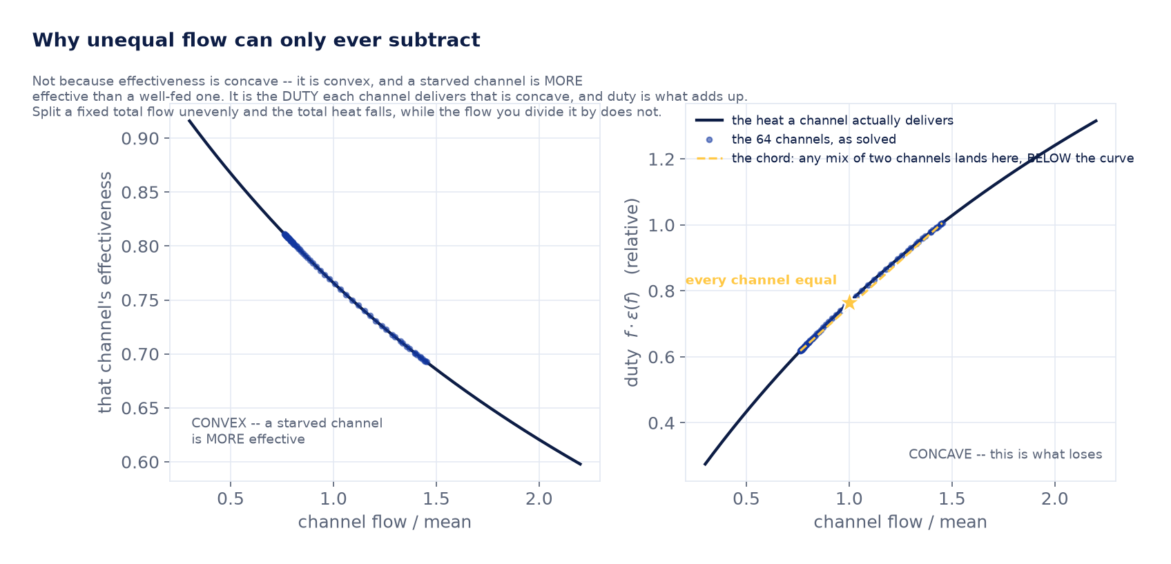
The intuition most people reach for here is wrong, and the correct version is more useful. A starved channel is more effective, not less: less air over the same plate area, more time to exchange heat. Effectiveness is convex in flow.

What matters is not effectiveness but the heat each channel actually delivers, which is its flow times its effectiveness — and that is concave. Split a fixed total flow unevenly and the total heat falls, while the flow you divide it by does not. So the stack effectiveness drops. Maldistribution can only ever subtract, but it subtracts through the duty, not through the effectiveness curve.

Effectiveness is convex; duty is concave — Left: a single channel's effectiveness against its flow — convex, so the starved channels really are the effective ones. Right: the heat that channel delivers — concave, and the chord between any two channels lands below the curve. That gap is the loss.

A prediction, and what it was worth

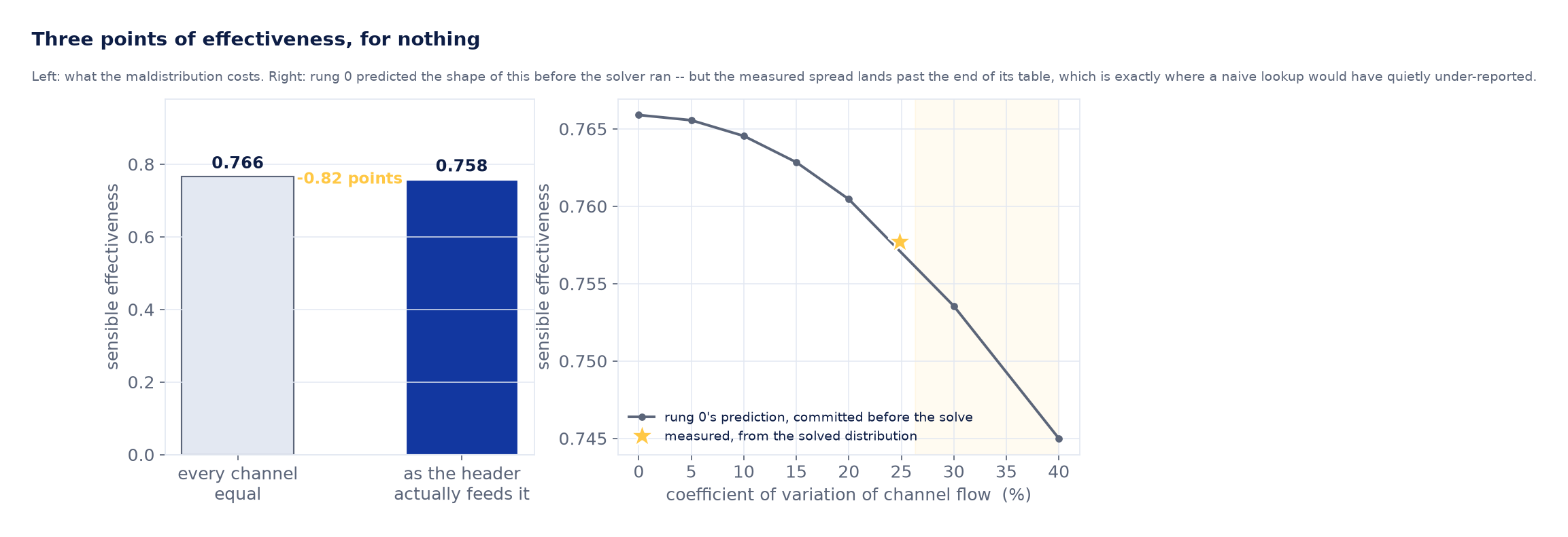
Effectiveness cost against the predicted curve — Left: what the maldistribution costs. Right: the penalty curve written down before the solver ran, against the solved point.

The penalty curve was committed in advance, parameterised by the one quantity the closed form could not supply: the spread in channel flow. At the solved spread of 25 % it reads 0.757. Computed instead from the actual solved distribution, channel by channel, the answer is 0.758. The prediction lands within 0.0006 of the solved value. That is the outcome worth having, and it says something precise: the closed form was never wrong about the consequences of maldistribution, only silent about the amount.

0.82 points is modest, and saying so is more useful than inflating it. On this geometry the header costs under a point of effectiveness — real, worth knowing, and smaller than the swing that rides on the Nusselt-number choice further up this page. The value of the CFD here is not that it found a catastrophe. It is that it turned an unbounded assumption into a bounded number, and the number happens to be small. That is a perfectly good answer, and it is only available once somebody solves for it.

What would move it

The shape of the curve says where the leverage is. The spread comes from the plenum being too small to let the air slow down before it has to turn, so the levers are the ones that buy deceleration: a deeper plenum, a plenum that tapers as flow is bled off along it so the remaining air holds a constant velocity, or a perforated distributor that trades a deliberate pressure drop for an even one. All three spend fan power to buy uniformity, and on these numbers that trade needs care — 0.82 points of effectiveness is not much to buy with a pressure drop when the core itself only costs 29 Pa.

This study solved one geometry and tested none of those, so none of them is a claim here. What it provides is the instrument: the same model with the same read-out answers each variant in a couple of hours, and the comparison is like for like because the spread is read the same way every time. That is usually more valuable than any single number — a rig you can ask the next question with.

Only the supply stream is in the domain. The exhaust slots are fed from the other end of the machine and appear here as solid walls, which is right for resolving how the supply header divides its air and useless for anything about the exchange itself. No heat transfer is solved at all. The effectiveness numbers come from applying the closed form channel by channel to the computed flow split — the CFD supplies the one thing the closed form cannot, and the closed form does the rest. That division of labour is the method, not a shortcut, but it does mean nothing here validates the thermal side.

It is also a two-dimensional section, so it contains the mechanism that matters — a plenum sharing flow between parallel channels — and nothing about the third direction, where a duct of finite width and the corners of the face do something this section cannot show. And one turbulence model spans a plenum at Reynolds ~32,000 and channels at Reynolds 501; k-omega SST integrates to the wall and collapses toward laminar where production is small, which is the standard choice, but the channels are not resolved the way a dedicated laminar solve would resolve them.

Revisions

v2 · Internal reviewThe 25% spread was redefined as a coefficient of variation, the 77% recovery relabeled as the ideal rating rather than a result, and 'measured' wording replaced with 'solved'.

Honest scope. Two-dimensional steady solve of one inlet plenum and all 64 supply channels together, k-omega SST, 69,216 cells, air at constant density, exhaust slots treated as solid. Inlet velocity derived from the real duct duty; the solve refuses to run unless its per-channel velocity matches the closed form's 1.81 m/s within 2 %. Channel flows are integrated node-by-node at mid-core by Simpson's rule; continuity is checked against the inlet plane integrated the same way and closes to 5.0 %, the residual being cell-to-node averaging on a seven-node channel. That bias is uniform across channels — changing quadrature moves the spread by less than one part in ten thousand — so it cancels in every ratio quoted here. Convergence is judged on the flux ratio ceasing to change, not on scaled residuals, which declared this case converged after 45 iterations. Effectiveness is not solved: it is the closed form applied per channel to the computed split, at a single Nusselt number, so that choice cancels in the penalty even though it does not cancel in the absolute effectiveness. No condensation, no latent recovery, no fouling, no frost, and no third dimension.

Have a device whose rating assumes something the geometry has to deliver? Plate exchangers, manifolds, catalyst beds, cold plates, battery packs — the design equations for all of them assume a flow split that a header has to actually provide, and the assumption is usually invisible in the calculation that depends on it. Finding out what your header really does is a couple of days of work, and it either confirms the rating or bounds the shortfall you have been arguing about. We do this work in Ansys Fluent and across the Ansys structural, fluids and electromagnetics tools. Rand Simulation — innovation through insight.