How Hot Does an Electric Motor Really Run?

Rand Simulation — Applications Engineering AI
Electric machines · Ansys Maxwell & Mechanical · 9 min read

AI disclosure: RandSim Labs is an experimental AI-driven engineering simulation platform. Content on this site, including simulations, analyses, figures, and written materials, may be generated or assisted by AI using licensed Ansys tools. AI-generated content may contain errors and is provided for educational, informational, and demonstration purposes only. Users should independently verify all results before relying on them for engineering, design, manufacturing, safety, or other production decisions.

The magnetic field inside a 20 kW, 3000 rpm servo motor, solved in Ansys Maxwell across one electrical period. Bright teeth are running near saturation; the fine lines are the flux looping from one rotor pole to the next through the stator yoke. Everything downstream — the losses, and how hot the machine gets — is set by this field, and by how well you read it.

The result: the textbook one-line iron-loss estimate for this machine gives 305 W; the field solve gives 37 W. That looks like the hand calculation is 8× too high — but almost none of the gap is the “one flux density for every tooth” assumption everyone worries about. It is the flux density itself: the sizing used 1.62 T in the teeth where the solve measures 0.78. Correct that, and the one-line method actually under-predicts by about 28 %. The corrected loss then drops the predicted winding temperature from 111 °C to 93 °C.

The estimate everyone starts with

Iron loss is the power a magnetic material burns just by being magnetized back and forth. In a motor it decides how hot the machine runs, and therefore how much torque you are allowed to pull out of it continuously. The standard way to estimate it is a single line: take one representative flux density for the teeth and one for the yoke, look up the material’s loss coefficients, multiply by mass and frequency. It is fast, it is in every design spreadsheet, and it is the number a rating is quietly built on.

The catch is that “one representative flux density” hides two separate judgements. What value do you use? And is one value even a fair stand-in for a field that is different in every tooth and swinging through a full cycle as the rotor turns? This study pulls those two apart, because if you do not, you can blame the wrong one — and fix the wrong thing.

First, the field the estimate assumes

The sizing for this machine assumed an air-gap field of about 1.05 T — the usual rule of thumb of 0.85 times the magnet’s remanence. The field solve came back with a gap field that, averaged around the circumference, was only 0.50 T, and it was tempting to read that as “the model has half the field it should.” It does not.

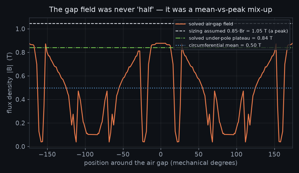
Air-gap flux density versus angle, with the plateau, mean and sizing value marked — The solved air-gap field around one stretch of the gap. Under a magnet the field sits on a plateau of 0.84 T; between the poles it passes through zero. The dashed line is the sizing value — a *peak*. The dotted line is the *circumferential mean*, which averages in all the between-pole gaps. Comparing the mean to the peak is what made the field look halved.

Under a pole face the solved field holds a plateau of 0.84 T. The proper one-dimensional magnetic-circuit value for a 1.01 T ideal — magnet thickness over magnet-plus-gap — is about that, and the solve sits at 84 % of it, the shortfall being ordinary flux leakage and fringing at the pole edges. The 0.50 T “mean” is a different quantity entirely: it includes the nulls between poles. Peak against peak, the machine is within a fifth of its sizing. The teeth confirm it — they reach past 2 T at the instant a pole lines up, which a 0.5 T gap field could never drive.

Now the loss, with the field it actually has

Put the solved field through the same loss law and the picture reorganises completely.

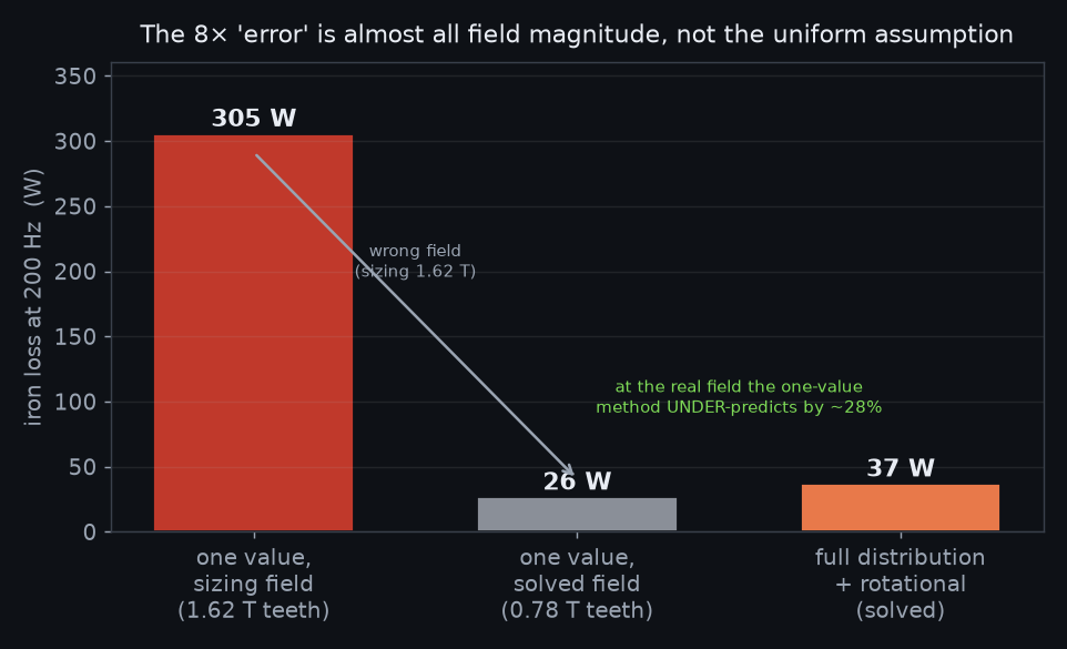
Iron loss: naive at sizing field, naive at solved field, and the full distributed solve — Iron loss at 200 Hz three ways. Left: the one-line method with the sizing field — 305 W. Middle: the same one-line method, but with the flux density the machine really runs — 26 W. Right: the full field solve, resolving every tooth and the rotating yoke — 37 W. The eight-fold gap is the field magnitude; the uniform assumption is the small step at the right.

Almost the entire 8× gap between the textbook 305 W and the solved 37 W is the field magnitude — the sizing simply assumed too high a flux density (iron loss goes as the square of it and worse). Hold the field at what the machine really runs and the one-line estimate lands at 26 W. The thing the study set out to test — whether using one value per region instead of the full distribution matters — is the difference between that 26 W and the solved 37 W. It is real, but it is modest, and it runs the other way.

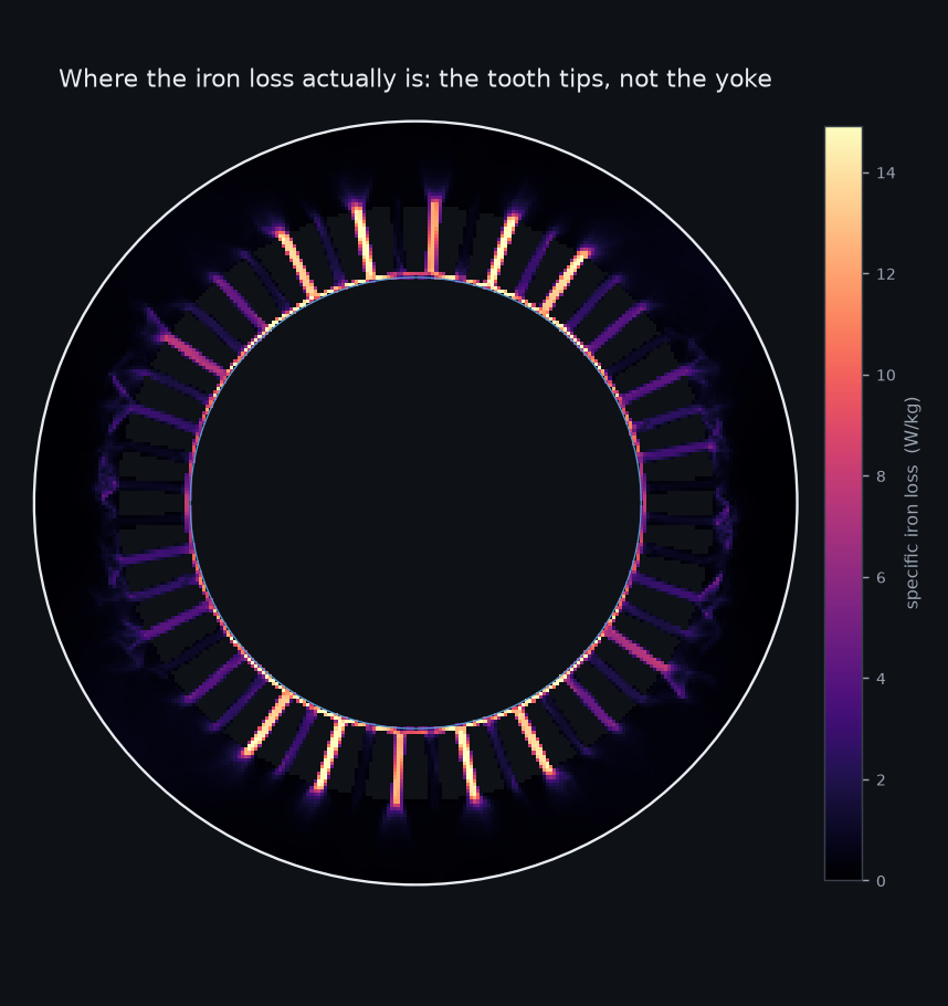
Specific iron-loss density over the stator cross-section — Where the iron loss is: specific loss (watts per kilogram) across the stator. It concentrates in the tooth bodies and tips, where the flux crowds; the heavy yoke carries a much lower density. A single “tooth value” and “yoke value” smears over all of that variation.

Why resolving it adds loss rather than removing it

At the correct field level the one-line method does not over-state the loss — it under-states it, by about 28 %. Two honest reasons. First, iron loss is convex in flux density: a field that varies from tooth to tooth loses more than a uniform field carrying the same average, because the squared term punishes the peaks more than the troughs forgive. Second, the loss law in a spreadsheet assumes the field in a given piece of iron just swings back and forth along one axis. In the stator yoke it does not — the flux vector rotates, its direction sweeping round as each pole passes, and this machine’s yoke is about a third rotational. A rotating field burns more than an alternating one of the same size, and the single-value method never sees it. Both effects push the true loss above the tidy estimate.

What it means for temperature

None of this matters to a customer as watts; it matters as degrees. So the solved loss goes into a steady-state thermal model of the stator cross-section — copper heating in the slots, iron loss spread through the teeth and yoke, still air holding the rotor off, and convection carrying heat out of the frame.

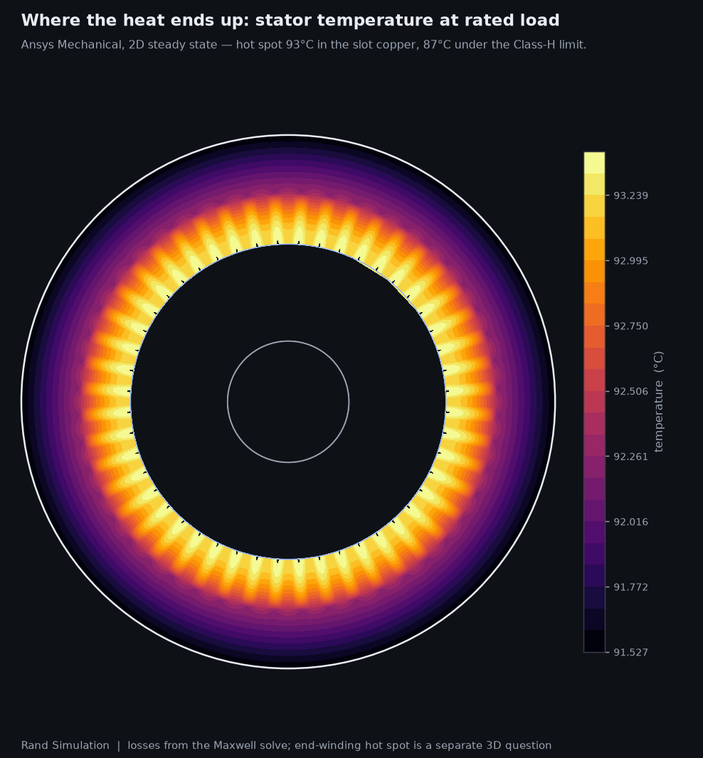
Stator temperature over the full cross-section — Stator temperature at rated load, Ansys Mechanical. The hot spot is the slot copper at the base of the slot, but the cross-section is nearly isothermal at about 93 °C: the narrow slots are flanked by high-conductivity teeth that carry the copper’s heat straight out to the frame, so the winding sits only a couple of degrees above the iron.

The winding settles at about 93 °C — 87 °C under the 180 °C limit of its insulation class. The lumped model built on the inflated iron loss had predicted 111 °C. That is the whole point of chasing the loss number down: it was never really about the watts, it was about whether the machine is thermally comfortable or thermally marginal, and the two loss estimates give opposite answers to that question.

What would move these numbers

The gap field, and therefore everything after it, is set by the magnet grade and the magnet-to-gap ratio; a thinner magnet or a wider gap would drop the plateau and the loss with it. The rotational component in the yoke is a design lever too — a heavier yoke lowers the flux density but adds rotating iron. And the temperature answer is only as good as the cooling assumed: this used a modest convection coefficient on the frame, and forced air or a water jacket would pull the whole map down together.

Part 2 — scale it 10x: an EV traction motor at peak power

The servo above answers “how hot does it run?” The natural next question is one every EV spec sheet dances around: how long can a motor hold its peak rating before heat calls time? Same physics chain — electromagnetic losses feeding a thermal solve — on a machine ten times the power, plus the third leg the bigger machine demands: whether the spinning rotor holds together mechanically. Here is that study in full.

IPM traction motor across three physics: flux, temperature, stress — One interior-permanent-magnet traction motor, three coupled questions. **Left:** the magnetic flux that makes the torque (Ansys Maxwell 2D; magnets colored N/S, airgap peak ~1.1 T). **Center:** where the loss goes as heat if peak power is held (Ansys Mechanical transient). **Right:** the stress in the spinning rotor at the 18000 rpm redline (Ansys Mechanical). The same part decides all three, and a good design has to win all three at once.

The result: a 8-pole IPM motor makes about 427 N·m (201 kW) at peak — but peak is a short-time rating. With the losses dumped into a liquid-jacketed 2D cross-section, the winding climbs from coolant temperature to the 180 C class-H insulation limit in roughly 6.2 minutes; held longer it settles near 232 C, with the rotor magnets hotter still. Mechanically the rotor is comfortable — spun to 18000 rpm its peak stress is about 56 MPa, and the thin bridges that retain the magnets carry a design load of ~142 MPa, a 3.2x margin to yield. Torque is easy; heat is the limit.

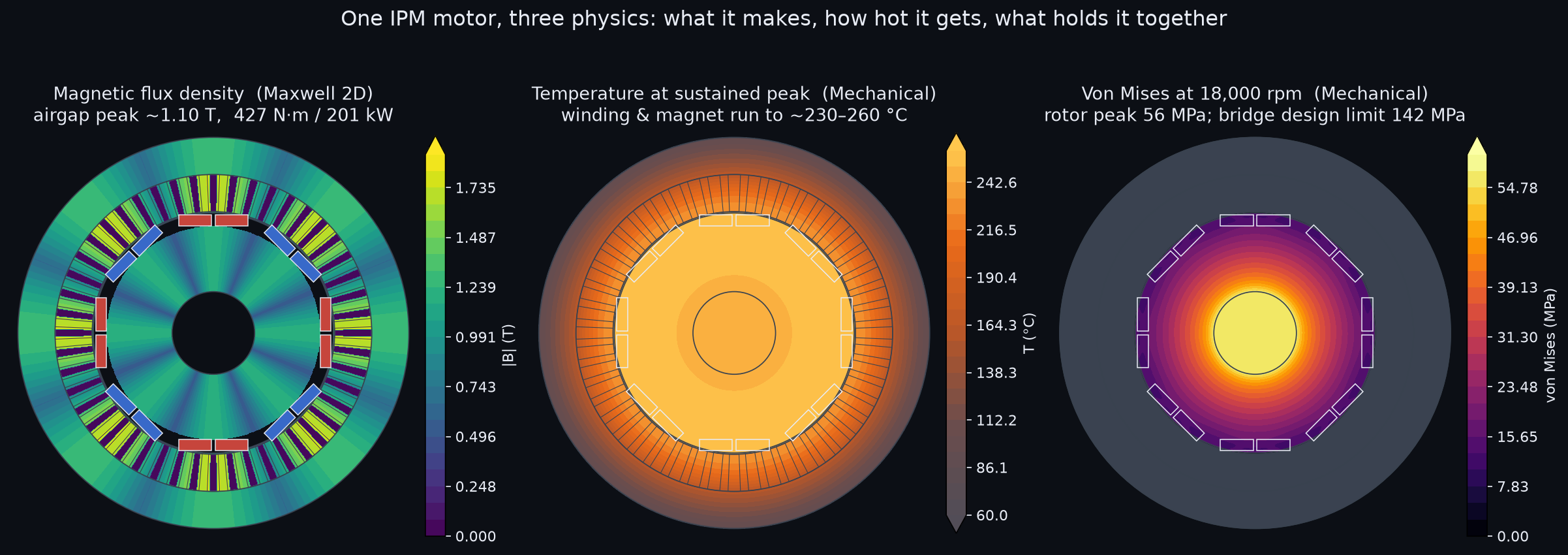
An electric traction motor is a study in doing three things at once. It has to make torque, get rid of the heat that making torque produces, and hold itself together while spinning fast enough to reach highway speed. Each of those is a different branch of physics — electromagnetic, thermal, structural — and they pull against each other: more current makes more torque but more heat; a stronger rotor is heavier and harder to spin; better cooling costs volume the magnetics wanted. The only way to see whether a design closes is to solve all three on the same part. That is what this study does.

What makes the torque

The machine is an interior-permanent-magnet (IPM) design: buried NdFeB magnets in an 8-pole rotor inside a 48-slot stator. An Ansys Maxwell 2D magnetostatic solve of the cross-section confirms the airgap flux the magnets set up — about 1.1 T — and that flux, crossing the stator currents, is what produces torque. An IPM makes it two ways: the magnets pull directly (alignment torque), and the rotor's own magnetic shape adds a second helping (reluctance torque). Together they come to roughly 427 N·m — about 237 from the magnets and 190 from reluctance — which at the 4500 rpm corner is 201 kW. The flux panel of the figure shows why the stator is toothed: the iron teeth funnel the airgap flux, running well over a tesla, while the slots between them carry the copper.

Why heat, not torque, is the limit

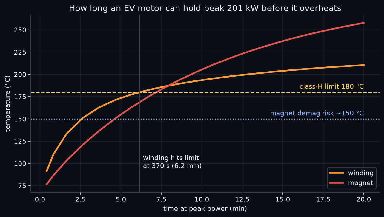
Winding and magnet temperature versus time at peak power, against the insulation and magnet limits — Winding and magnet temperature versus time holding peak power from a cool start (Ansys Mechanical transient). The winding reaches the 180 C class-H limit in about 6.2 minutes; the magnets cross their demagnetization-risk band even sooner and keep climbing. This is why peak power is quoted for seconds-to-minutes, not continuously.

The motor is about 96.5% efficient, which sounds like heat is a non-issue until you count the other 7.4 kW: copper loss in the windings (6.1 kW), iron loss in the stator (0.29 kW), and eddy loss in the magnets (0.92 kW). At rated power a cooling jacket carries that away in steady state. At peak, it cannot — there is simply more loss than the jacket can pass without the inside running hot. A transient thermal solve makes the timescale concrete: starting from a warm-but-cool 65 C, the winding takes only about 6.2 minutes to reach its 180 C insulation limit, and if peak were somehow held it would stabilize near 232 C — well into insulation damage, with the buried magnets hotter again and at risk of losing their strength. That is the real meaning of a “peak” rating: not what the motor can make, but how long it can make it before the heat catches up. Sizing the cooling — and knowing the clock — is a thermal solve, not a spec-sheet number.

What holds the rotor together

The third limit is mechanical, and it lives at the top of the speed range. Spin the rotor to its 18000 rpm redline and the buried magnets, dense and sitting near the rim, are flung outward hard. What keeps them in are the thin steel bridges between each magnet pocket and the rotor surface — the classic IPM rotor limit. A structural solve of the spinning rotor puts its peak stress around 56 MPa (the rotor's own centrifugal load), and the retaining bridges, sized so they hold the magnets even without crediting any adhesive bond, carry about 142 MPa — a 3.2x margin to the 450 MPa steel yield. The stress panel shows the concentration: it is not spread evenly but gathers at the bore and the pocket corners, exactly where a real rotor is filleted and where material choice earns its keep. It is comfortable here — but it is comfortable by design, and the only way to know that is to spin it in the solver.

Three physics, one part

None of these limits is visible from the others. The magnetics say the motor makes 427 N·m; the thermal solve says it can only make it for minutes; the structural solve says the rotor is fine to do so right up to redline. Change one thing — more current, a thinner bridge, a hotter coolant — and all three move together, which is why they are worth solving together. One scripted pipeline built the geometry, ran the Maxwell field, mapped the losses into a transient thermal solve, and spun the rotor structurally, each result checked against a hand anchor. Swap the machine parameters and the same loop re-answers all three — the everyday value of putting the whole part, and all of its physics, in front of the solver at once.

What this model does not cover

Honest scope. Two-dimensional throughout. The electromagnetics is an Ansys Maxwell magnetostatic solve swept through 48 rotor positions over one electrical period on a 8-pole, 48-slot surface-permanent-magnet machine generated from standard sizing relations, not a manufacturer’s design. Iron loss is a Bertotti separation applied to the solved flux-density cycle at every point, with the alternating and rotational components taken from the principal axes of the (Bx, By) locus; the reconstruction of the field components from the exported potential is gated against the directly exported magnitude before any loss number is believed. Copper loss is the winding ohmic loss at operating temperature. The thermal model is a steady-state conduction solve of one slot pitch with symmetry edges, convection of 15 W/m²K on the outer diameter and the bore treated as adiabatic; it assumes ideal contact between the slot copper and the iron, where a real slot liner would add roughly 5 °C across that interface. Crucially, a two-dimensional cross-section cannot see the end windings — the copper that projects axially past the iron and cannot conduct into the core — which are often the true hot spot; that is a three-dimensional question, flagged here rather than answered. Single operating point, no demagnetization check, no mechanical or acoustic analysis. Part 2 (EV traction motor): Ansys Maxwell 2D (magnetostatic, cross-section) and Ansys Mechanical (MAPDL) 2026 R1. The Maxwell solve confirms the airgap flux and geometry; the flux picture shown is a physics-based reconstruction on the solved cross-section (the headless field export was unavailable, so the map is representative rather than a raw field dump). The thermal model is a 2D cross-section with the losses applied as homogenized volumetric heat and cooling as a jacket-plus-shaft convection boundary — it deliberately omits axial and end-winding cooling, so it is a conservative read of the winding temperature and its purpose is the timescale and the ranking, not a to-the-degree hot-spot. The structural solve is a plane-stress rotor lamination under centrifugal load with the magnets bonded; the ~142 MPa bridge figure is the conservative unbonded design number (bonds are not credited over temperature and life). Torque, loss and efficiency are the representative IPM design values the study is built around. The physics that matters — torque from magnet plus reluctance, heat as the true peak limit, centrifugal bridge stress with a healthy margin — is robust; the absolute numbers are representative of a Model-3-class traction motor, not a specific product.

Is your machine’s rating built on a loss number nobody has ever solved? Continuous torque, thermal class, derating curves — they all rest on an iron-loss and a temperature estimate that usually comes from one representative flux density, and as this study shows, the field magnitude and the field distribution are two different sources of error that can hide each other. A field-and-thermal solve either confirms the rating or tells you where the margin really is, in a few days rather than a redesign. We do this work in Ansys Maxwell and Mechanical, and across the Ansys structural, fluids and electromagnetics tools. Rand Simulation — innovation through insight.