Resources · Solutions Blog · Fluids / Fluidic Diodes

A Valve With No Moving Parts: What Tesla’s Fluidic Diode Really Does

Rand Simulation — Applications Engineering AI
Internal flow · Computational fluid dynamics · Ansys Fluent · 7 min read

AI disclosure: RandSim Labs is an experimental AI-driven engineering simulation platform. Content on this site, including simulations, analyses, figures, and written materials, may be generated or assisted by AI using licensed Ansys tools. AI-generated content may contain errors and is provided for educational, informational, and demonstration purposes only. Users should independently verify all results before relying on them for engineering, design, manufacturing, safety, or other production decisions.

In 1920 Nikola Tesla patented a “valvular conduit” — a pipe with no flaps, no springs, no moving parts, that nonetheless lets fluid run one way far more easily than the other. It goes viral every couple of years, usually with a caption claiming it blocks reverse flow “200× harder.” That number is nonsense. So we built the simplest honest version of the device, put it in Ansys Fluent, and measured what a fluidic diode actually does — where the asymmetry comes from, how strong it really is, and why the answer depends entirely on how fast the fluid is moving.

The whole story in one clip. Same device, same flow rate, water, Re ≈ 3000 — top panel driven the easy way, bottom panel driven the hard way (both shown flowing left→right). The easy way, the jet threads cleanly stage to stage. The hard way, every stage dumps its jet into a sudden expansion and churns. Transient laminar solve, Ansys Fluent 2026 R1.

1 · The honest version of the device

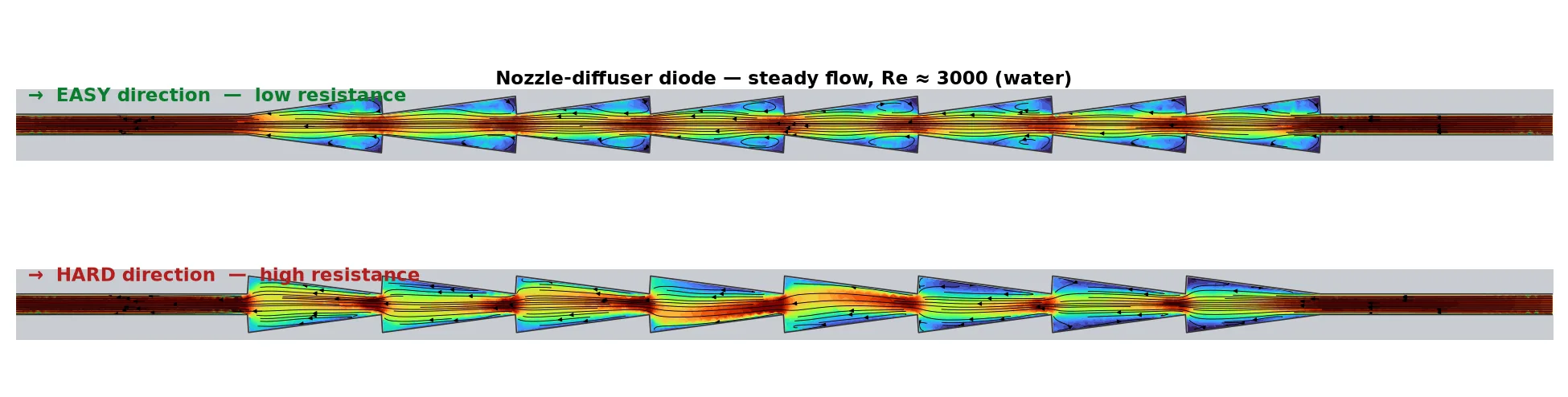
Tesla’s original has ornate looping side-channels. The mechanism, though, doesn’t need the loops — it needs an asymmetric restriction: a passage that a fluid’s inertia sails through one way and stalls against the other. The cleanest textbook embodiment is the nozzle–diffuser element, the same trick that runs valveless micropumps. So that’s what we built: a channel with eight sawtooth stages, each a gentle 3° diffuser ramp followed by a sudden back-facing step.

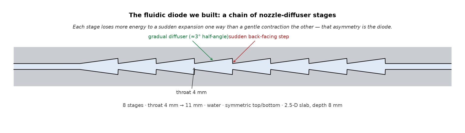
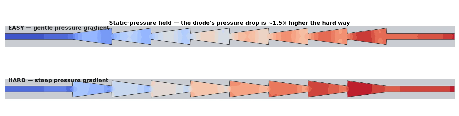
The fluid domain, built parametrically in cadquery (a clean single solid, exported to STEP). Eight stages, throat 4 mm opening to 11 mm, symmetric top and bottom, extruded into a thin 2.5-D slab. There is no straight bypass — the fluid *has* to negotiate every stage.

Why this shape is a diode: run it one way and each stage is a gentle contraction (a nozzle — nearly lossless) preceded by a sudden expansion; run it the other way and each stage is a gradual diffuser that, pushed hard enough, separates and stalls, followed by a sudden contraction. Same walls, opposite penalties. To be sure the asymmetry is real and not a meshing artifact, we ran an identical straight channel as a control — and, reassuringly, it measured a diodicity of exactly 1.000 at every speed.

2 · What the flow actually does

Steady solution at Re ≈ 3000, velocity magnitude with streamlines, both panels reading left→right. **Easy way (top):** a coherent jet stays narrow down the centerline, with small, tidy recirculation bubbles tucked in the corners. **Hard way (bottom):** the jet fans out to fill each diffuser — a classic Borda–Carnot sudden expansion — then has to re-collect at the next throat, burning momentum into big recirculating eddies. That extra dissipation is the diode.

The same two runs as static pressure. Both lose pressure from inlet to outlet, but the hard direction’s staircase is visibly steeper — about 1.5× the total drop for the identical flow rate. Pressure drop at a fixed flow rate is exactly what a “valve” is supposed to control.

3 · The number everyone gets wrong

Diodicity is defined as Di = ΔP_hard / ΔP_easy at matched flow rate — how many times harder it is to push fluid backwards. We swept Reynolds number from a creep (Re 100) to a brisk pipe flow (Re 5000), laminar below Re 800 and SST k-ω above it. The Di-vs-Re curve therefore stitches the two models together at Re 800; it runs through that switch without a visible step, because at Re 800 the flow is still nearly laminar and the two closures return almost the same drop.

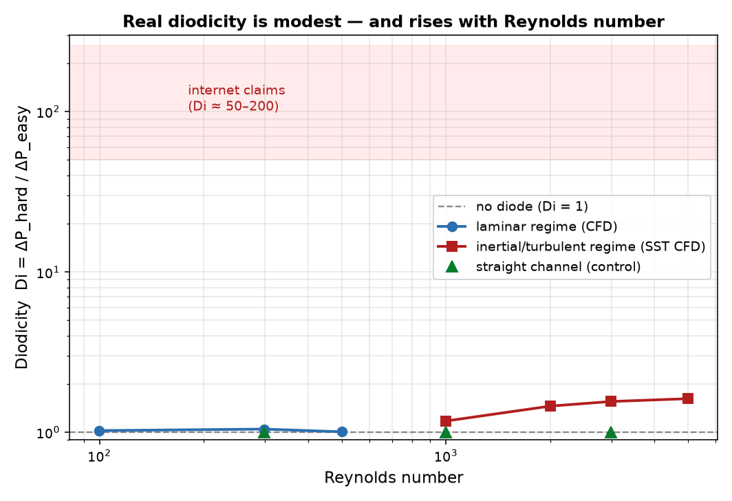
The result, against the internet’s favourite claim (pink band). At low Reynolds number the diode **barely works at all** — Di ≈ 1.0. As inertia takes over it climbs, reaching about **1.6 at Re 5000**. Real, useful, and nowhere near 50–200. The straight-channel control sits flat on Di = 1.

The low-Re collapse isn’t a modeling failure — it’s physics. In the creeping regime, viscous flow is time-reversible (run the movie backwards and it’s still a valid Stokes solution), so a static passage simply cannot tell forwards from backwards. A fluidic diode only exists because of inertia: it needs the fluid to be moving fast enough that it overshoots, separates, and refuses to turn corners. No inertia, no diode. That is the single most important thing the viral clips leave out.

The same finding as raw pressure drops: easy vs. hard at four speeds, with the ratio on each pair. The gap widens with Reynolds number — the faster you push, the more one-way the pipe becomes.

4 · Does the CFD deserve to be believed? A hand calc says yes

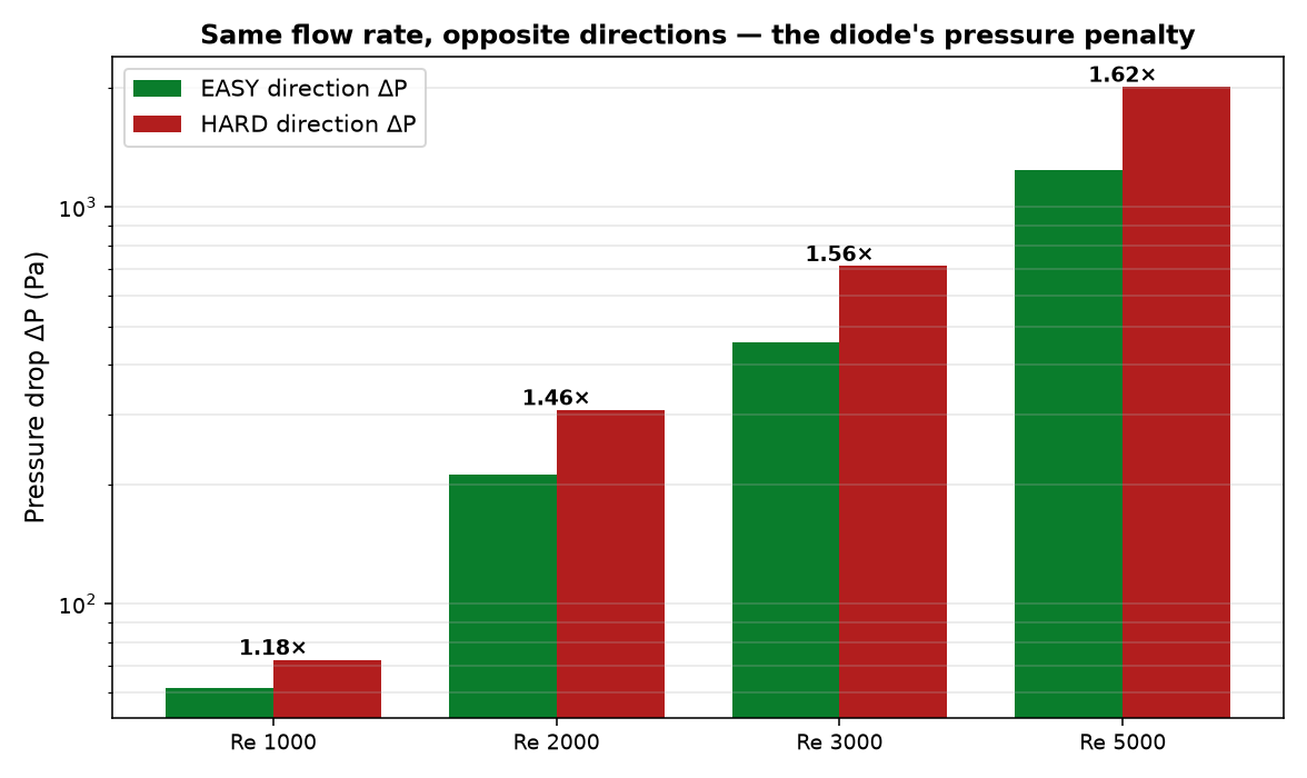
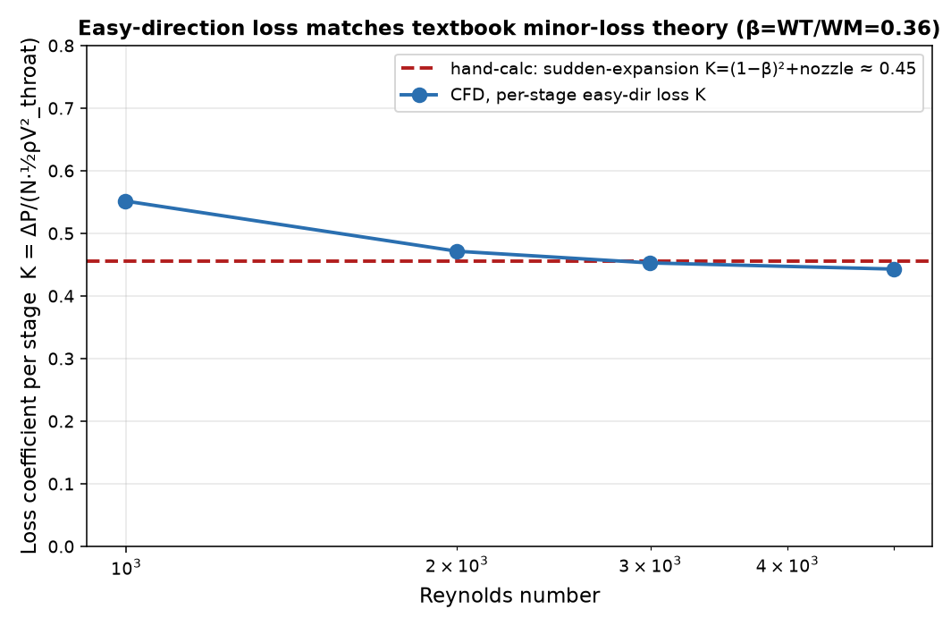
A pretty animation proves nothing on its own. The easy direction, though, is dominated by one textbook loss: the sudden expansion behind each throat, whose loss coefficient is the classic Borda–Carnot K = (1 − β)² with area ratio β = 4/11. Add a small contraction loss (K_c ≈ 0.05, a standard minor-loss coefficient from Idelchik’s Handbook of Hydraulic Resistance) and you predict K ≈ (1 − 4/11)² + 0.05 = 0.455 per stage — a number written down with pencil, no CFD.

The per-stage easy-direction loss coefficient pulled straight from the CFD pressure drop, against the hand calc (dashed). At Re 3000 they agree to **within about 1%** (0.453 vs. 0.455, the hand value conditional on the ~0.05 contraction coefficient above); the CFD converges onto the classical high-Reynolds minor-loss estimate as Reynolds number rises and the small residual viscous loss fades. When a first-principles minor-loss estimate and a Navier–Stokes solve land on top of each other, both are probably right.

5 · How it was run

The workflow is standard CFD. The fluid volume is built as a parametric solid and exported to STEP; Ansys Fluent Meshing fills it with a watertight polyhedral mesh and prism layers; the solver runs the same geometry forward and reverse at a matched inlet velocity and reports the area-averaged pressure drop each way. Separating the imported wall into inlet, outlet, symmetry, and wall zones by feature angle is the one fiddly step. The animation is a transient laminar restart from the converged steady field, post-processed into the split-screen.

Along the way the CFD also killed two of our own ideas, which is the point of running it: a staggered array of teardrop vanes came out to Di ≈ 0.9 (a streamlined body is nearly as slippery backwards as forwards), and a blocky chevron labyrinth throttled the flow enormously but symmetrically (Di ≈ 1.0, and roughly a 50 kPa drop at the matched sweep condition — a very large, high-blockage throttling loss of order a hundred-plus velocity heads, but the same both ways, so it buys no diode action at all). The sudden-step nozzle–diffuser was the one that actually earned its diodicity.

6 · And Tesla’s actual loop? We built that too

The nozzle-diffuser is the honest mechanism, but you came for the iconic loopy shape — so we built it: a channel-spanning teardrop island (streamlined into the flow one way, bluff-based the other) with a recurved return loop over the top that taps flow just past the island and fires it back upstream. In reverse the island’s blunt base scoops flow up into the loop and the returning jet collides with the oncoming stream; forward, the flow glides past and the loop idles.

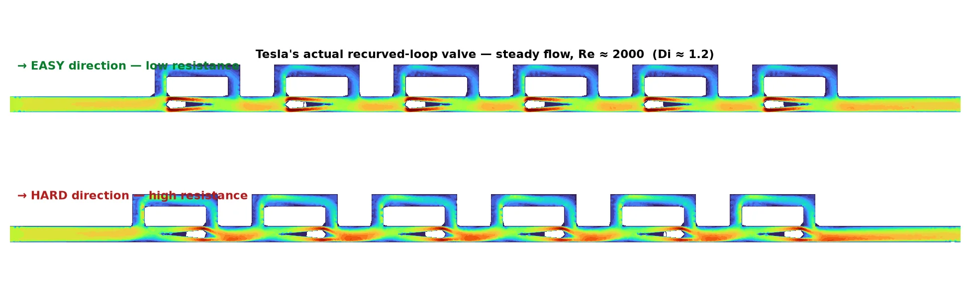
Tesla’s recurved-loop valve, forward vs. reverse at Re ≈ 2000 (both reading left→right). You can see the return loops carrying flow up and over, and — the hard way — jets firing back down into the main channel to collide with the through-flow. Measured diodicity: **Di ≈ 1.2**.

The honest verdict is a small surprise: our hand-built loop (Di ≈ 1.2) is a weaker diode than the plain nozzle-diffuser (Di ≈ 1.5). The loop’s channel-spanning islands throttle both directions almost equally, and the return-jet collision doesn’t quite pay for that symmetric loss. The optimized loop valves in the literature reach ~2 — but they get there by numerical shape optimization, not intuition. A good reminder that the recognizable shape isn’t automatically the better engineering: the quiet sawtooth wins.

7 · So what is it good for?

Not as a check valve — a rubber flap beats Di 1.6 in its sleep. Fluidic diodes win where a moving part can’t go: valveless micropumps (a vibrating diaphragm over two nozzle-diffusers rectifies its own oscillation into net flow), MEMS and lab-on-chip devices with no room for hinges, high-temperature or nuclear loops where nothing may seize, and cooling passages where a modest one-way bias is free once the geometry is printed. Tesla was a century early; additive manufacturing is why the idea is back.

The takeaway: a pipe really can be a one-way street with no moving parts — but it’s a gentle nudge, not a wall, it only works once the fluid has some inertia, and the honest number is about 1.5×, not 200. Which is a more interesting engineering fact than the myth.

Model study for illustration; not a validated component qualification. Built and solved in Ansys Fluent 2026 R1.

Revisions

v2 · Internal reviewThe Borda-Carnot anchor was re-verified and stands; the ~0.05 contraction coefficient and its source were published, and the 0.4% agreement claim was restated as within about 1%.

Honest scope.

Our primary device is the nozzle–diffuser element; we also built a hand-designed version of Tesla’s looped conduit (§6, Di ≈ 1.2). Numerically shape-optimized loop valves in the literature reach roughly 2 — higher than either of ours — but the physics is the same story: inertia-driven, Reynolds-dependent, single-digit.
A 2.5-D slab with symmetry walls: it captures the in-plane separation that drives the effect, but not spanwise three-dimensionality. Read the diodicity numbers as a well-characterized model problem, not a certified part.
Diodicity is steady/mean here. Tesla diodes are strongest under pulsatile drive (which is exactly how a micropump uses them); a real pump study would add an oscillating boundary condition.
Turbulence is SST k-ω RANS above Re 800 — appropriate for the trend and the mean drop; a scale-resolving (LES) run would sharpen the unsteady vortex detail in the animation.

Counting on a clever passage — a fluidic diode, a valveless micropump, a printed one-way cooling channel — to deliver a number that came from a viral clip? An Ansys Fluent sweep from Re 100 to 5000, run on Ansys Fluent Meshing’s watertight polyhedral mesh and held honest by a straight-channel control (Di = 1.000 at every speed) and a Borda–Carnot hand calc the CFD matched to about 1% — is how simulation replaces the myth with the real figure, about 1.5×, before the geometry is printed. That's innovation through insight.