Why Where the Pipe Enters Changes How a Tank Mixes
Sizing a completely-mixed tank is a one-line calculation: hydraulic retention time is volume over flow. For this 254 m³ contact/equalization tank at 1728 m³/day that is 3.5 hours — a routine operating point for that duty — and the whole design hangs off it: the contact time the water is credited with, the smoothing the downstream process counts on, the permit that cites the number. The model behind that line, the ideal continuously-stirred tank, says the distribution of residence times is a pure exponential set by nothing but the volume and the flow. It contains no term for where the influent pipe enters. Not a small term — none.
The mass balance comes before every other number
An RTD is a bookkeeping exercise before it is anything else: put a known quantity of tracer in, and account for all of it. Every case here closes to within 0.8 % — tracer out of the effluent plus tracer still inside the tank, against tracer injected. That check is not a formality. It is what separates a transport calculation from a plausible-looking picture, and it is the first thing worth asking of anyone's RTD, including ours.
It is also a check we needed. An earlier version of this model ran to completion with every residual converged and reported a tracer concentration of 1.5 × 10¹¹, growing steadily to the last timestep. The scalar transport equation had been set up without its time derivative, which on a recirculating domain makes it singular — any constant satisfies it — so the solver simply drifted, converging beautifully at every step. Nothing in the solver output says the equation is the wrong one. The mass balance says it immediately.
| influent depth | mass closure | out by θ = 0.2 | mean residence | still held at θ=6 vs ideal | bottom third |
|---|---|---|---|---|---|
| 4.5 m | 1.008 | 44 % | ≥ 0.95 τ | 10× | 19 % |
Nearly half the slug leaves in a fifth of a residence time
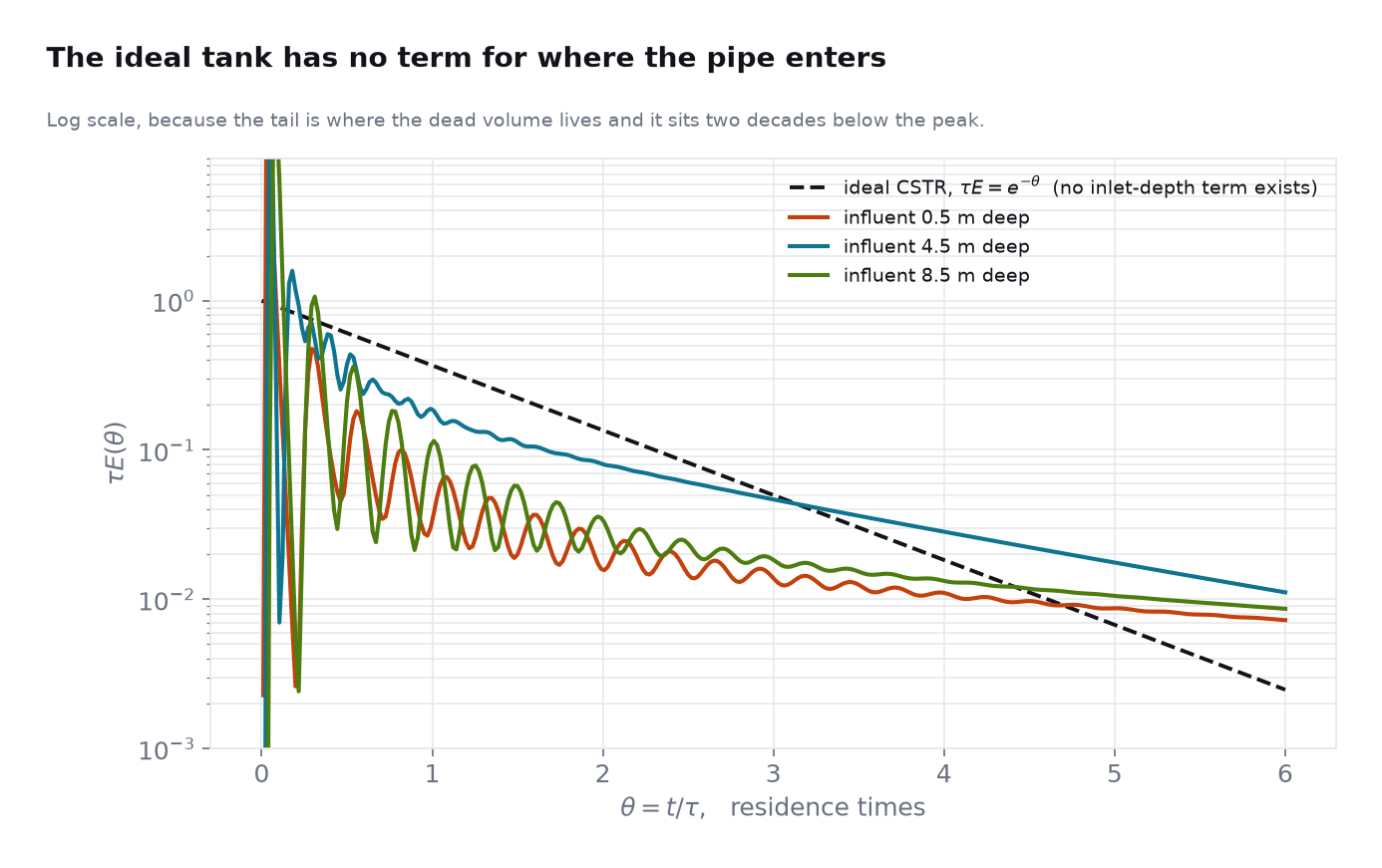
The shape is the classic signature of a tank that is not doing what its nameplate says. A spike far too early, then a middle section running below the ideal because that tracer has already gone, then a tail running above it because what is left is stuck. Cumulatively the early part is stark: 44 % of the slug is out at θ = 0.2 in the worst case, against 18 % ideal.
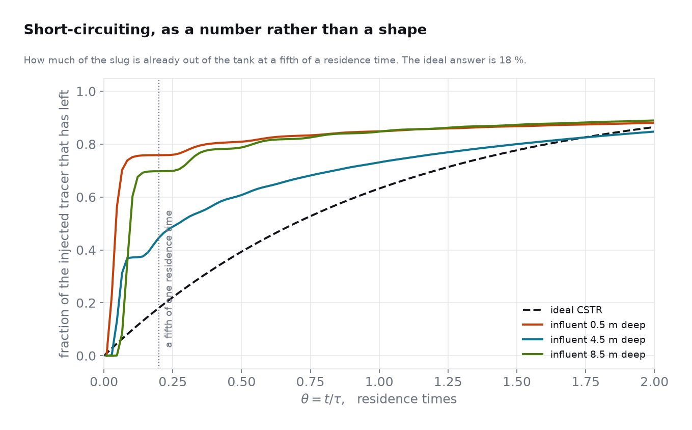
For a contact or equalization tank this is the number that matters, because it is fluid that has spent only a fraction of the design retention time in the vessel and has then left — credited, on paper, with the full 3.5 hours. Hydraulic retention time is a mean, and a mean is a poor description of a distribution with a spike at one end.
The dead volume, without extrapolating anything
The obvious next step is to integrate the distribution for the actual mean residence time and call the shortfall against V/Q dead volume. That step is a trap, and it is worth showing rather than hiding, because the trap is generic to every pulse test ever run — in CFD or in a real tank.
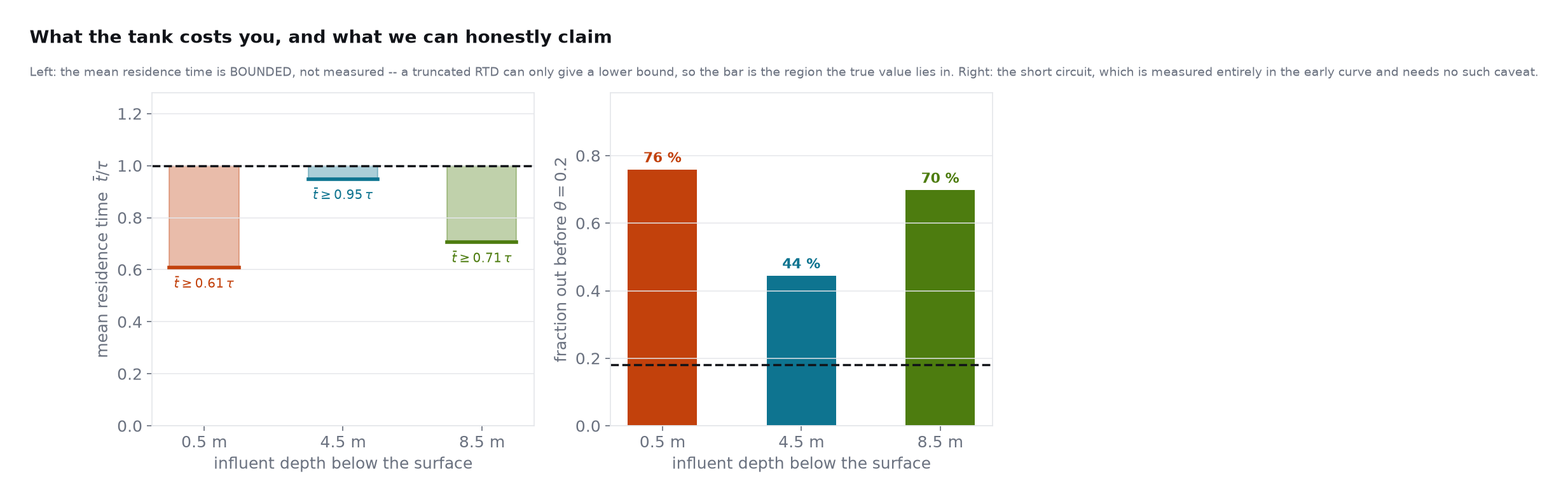
A finite test is truncated by definition. Every gram of tracer still inside when you stop measuring will leave later and would have added to the integral, so the integral you have is a lower bound on the true mean, and any dead-volume figure it implies is an upper bound. At four residence times this study still had 6 % of the tracer inside, and that 6 % was the difference between claiming 38 % dead volume and being able to defend 13 %. The runs go to six residence times for that reason.
Going longer helps less than you would expect, and the reason it helps less is itself the answer. An ideal tank holds e−6 — 0.25 % — of the tracer after six residence times. This one still holds 2.5 %, which is 10 times as much. Nothing in that comparison is extrapolated, fitted or integrated past the data: it is the amount of dye left in the tank at the moment the run stopped, against the amount an ideal tank would have. The fluid that is stuck is genuinely stuck, and that is why no practical test length will ever pin the mean down tightly.
Which third of the tank sees the feed
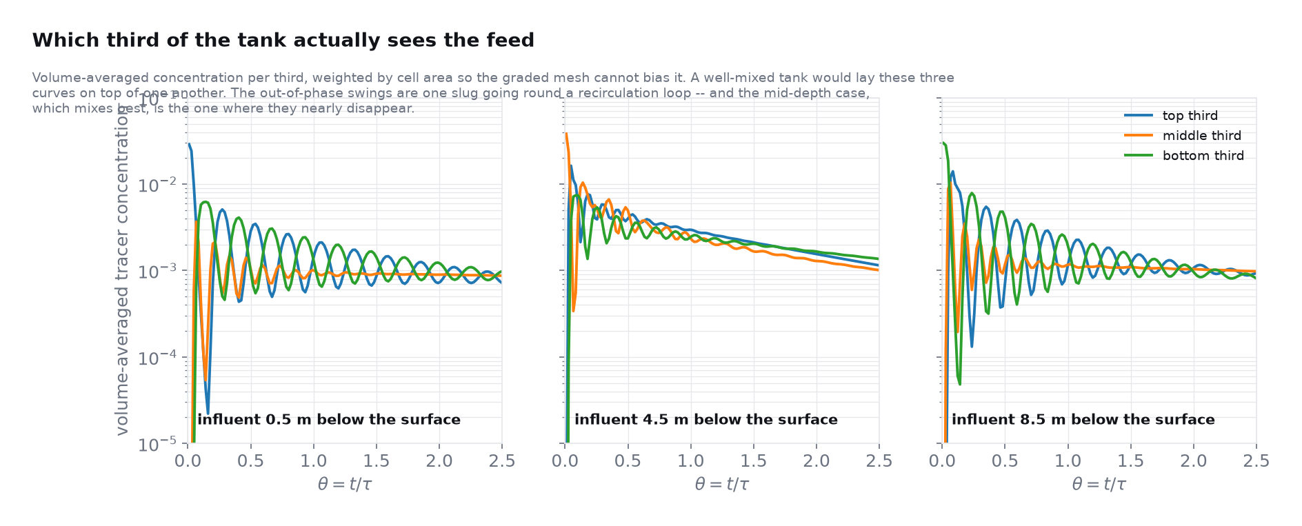
They do not lie on top of one another. With the influent 4.5 m below the surface the middle third peaks highest and the bottom third reaches only 19 % of it. A CSTR model cannot represent this at all: it has one concentration, everywhere, by construction. The practical consequence is that the volume you built to provide retention is not the volume that is doing the work.
The effluent signal has a heartbeat
Riding on every one of the distributions is a regular ripple, and it is worth a paragraph because the first job was to prove it is not an artifact. The snapshots are 6 s apart, so anything with a period under 12 s would alias into something spurious. It is not that: the period comes out at 7 to 7 samples, far above that limit, and — the decisive part — it changes with the inlet depth, 42 s at 4.5 m. A fixed sampling cadence cannot produce a period that tracks a boundary condition.
What is left is the physical reading: the tank runs a large recirculation cell, and a parcel of tracer passes the effluent weir once per lap. The period is the circulation time, and the amplitude is how coherently the cell holds together. The best-mixed case has both the shortest period and much the weakest ripple — the same jet that entrains instead of hugging a wall breaks one big loop into smaller ones, and that is visible in the outlet signal without looking at the flow field at all.
What this model cannot tell you
The tank is modeled as a vertical slice through the diameter, and that choice is deliberate: an axisymmetric model would put the influent on the centerline by construction and could not represent an off-axis feed at all — it would answer a different question and look rigorous doing it. But a slice gives up swirl and everything azimuthal, and a real circular tank with a tangential feed has both.
The slice also carries its own retention time rather than the tank's, so all of the above is reported against θ = t/τ of the model. The direction of that bias is worth naming: relative to the real tank the slice gets far more jet momentum per unit of throughflow, so it is biased toward looking well mixed. The short-circuiting it finds anyway is a floor, not a ceiling.
Two of the five questions written down before the solve are outside it. The mesh has a single exit, so we cannot compare an RTD measured at the top of the tank against one measured at the bottom — the band concentrations above are the closest the geometry can get. And the solids are not modeled: whether near-neutrally-buoyant particles track the liquid or slowly accumulate on the floor over many retention times is a discrete-phase question, and a passive scalar cannot answer it.
Have a vessel whose nameplate retention time you have never actually checked? Digesters, clarifiers, contact tanks, chlorine basins, thickeners — the design equations for all of them assume a mixing state that the geometry has to deliver, and the cheapest way to find out whether it does is a tracer study, real or computational. The interesting output is rarely the mean; it is the fraction that leaves early. We do this work in Ansys Fluent and across the Ansys structural, fluids and electromagnetics tools, and we are happy to talk through whether a CFD tracer study or a field test is the right instrument before anyone commits. Rand Simulation — innovation through insight.