How a Thermal Solver Repairs a Scratched Photograph

Rand Simulation — Applications Engineering AI
Image restoration · Ansys Mechanical · 8 min read

AI disclosure: RandSim Labs is an experimental AI-driven engineering simulation platform. Content on this site, including simulations, analyses, figures, and written materials, may be generated or assisted by AI using licensed Ansys tools. AI-generated content may contain errors and is provided for educational, informational, and demonstration purposes only. Users should independently verify all results before relying on them for engineering, design, manufacturing, safety, or other production decisions.

A scratched NASA portrait of astronaut Eileen Collins healing as a reveal sweeps across it. Left of the seam is the repaired photo, right of it is the damage, and the seam itself is the solved temperature field pouring into the gap. Every filled pixel is the steady-state temperature an Ansys Mechanical heat-conduction solve computed for that point, holding the surrounding healthy pixels as fixed temperatures. The photograph is public domain (NASA); the damage was added by us so we keep a ground truth to score the repair against.

The healing brush is secretly a heat problem

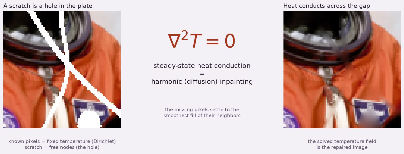
Almost everyone has used the “healing brush” or “spot heal” in a photo app to wipe a scratch, a dust speck, or a stray hair off a picture. Almost no one knows that, in its simplest form, that tool is literally solving a heat-conduction problem. Steady-state heat conduction with no heat source is Laplace’s equation, ∇²T = 0, and a photo editor fills a damaged patch by demanding exactly that of the missing pixels: let them settle to the smoothest values consistent with the healthy pixels around the edge, the same way temperature settles across a metal plate once the rim is held fixed.

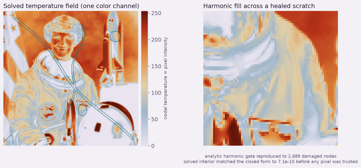
So we did the honest thing. We took a scratched photograph, called the damage a hole in a plate, pinned every healthy pixel around it as a fixed temperature, and handed the whole thing to a real Ansys thermal solver. We did not write the physics in Python and dress it up as a solve — the Ansys Mechanical solver assembled and solved the same Laplace operator it would for a heat-transfer job. The steady-state temperature field it returned is the repaired image.

One thing has to be said before the pretty picture, because it is the honest heart of the study: this equivalence is exact only for the diffusion family of healing — the classical kind that smooths a repair across a gap. It is not the “content-aware fill” in modern editors, which uses a completely different algorithm (PatchMatch texture synthesis) to copy real texture into the hole. Diffusion cannot invent texture. So a thermal solver erases a scratch across a cheek or a clear background beautifully, and it blurs a scratch that crosses hair or an edge. We show both, and we measure both.

The verdict. A steady-state heat-conduction solve genuinely repairs a scratched photo: the damaged pixels become the harmonic fill of the healthy pixels around them, and the reconstructed image scores 19.2 dB PSNR against the known original overall. But the quality splits exactly where the physics says it should — 26.3 dB across smooth regions (skin, the orange suit, the background) versus 18.0 dB across texture (the flag, hair, the shuttle), because diffusion smooths and cannot rebuild detail. The Ansys solve reproduces the exact discrete-harmonic inpainting a photo editor relaxes to within about one gray level, and it lands within a decibel of OpenCV’s own diffusion repair — so the “same equation” claim is measured, not asserted. What it cannot do — rebuild texture or a sharp edge — is what content-aware fill (a different, non-physics algorithm) is for.

Why heat conduction is the same math as inpainting

Steady-state heat conduction in a uniform plate with no internal heating obeys Laplace’s equation, ∇²T = 0. A function that satisfies it is called harmonic, and there is exactly one harmonic function that matches a set of values prescribed around the boundary of a region — its harmonic extension. Diffusion-based image inpainting is precisely that: fill the damaged region with the harmonic extension of the surrounding known pixels. Each filled pixel becomes a conduction-weighted blend of its neighbors, propagated inward from the healthy ring, with no bumps or kinks of its own. That is why a diffusion heal always looks smooth — smoothness is the equation’s only instruction.

A zoom of a scratch across the astronaut's suit, the heat equation, and the same patch healed. — The whole idea in one line. The scratch is a hole in the plate: the known pixels around it are held at fixed temperatures (a Dirichlet boundary condition), the scratched pixels are left free, and steady-state conduction settles them into the smoothest fill of their neighbors. The solved temperature field is the repaired image.

There is a subtlety worth naming rather than hiding. A photo editor’s diffusion fill uses the 5-point pixel Laplacian — each pixel is nudged toward the average of its four orthogonal neighbors. Our finite-element plate uses PLANE55 bilinear quadrilateral thermal elements, whose consistent stiffness matrix is a slightly different (nine-point-class) discrete Laplacian. Both are legitimate discretizations of the same continuous operator, and both converge to the same harmonic answer as the grid gets finer; they agree closely but not bit-for-bit. Rather than paper over that, we measured it.

Handing the photo to Ansys Mechanical

The image is a public-domain NASA portrait of astronaut Eileen Collins, chosen because a lay reader recognizes it instantly and because it carries both kinds of region we need: smooth expanses (skin, the orange launch suit, the studio background) and textured detail (the US flag stripes, hair, the Space Shuttle model). We worked at 256 × 256, which maps to a plate of 65,536 nodes and 65,025 PLANE55 elements — one node per pixel, numbered so that pixel k is node k is export row k. We synthesized the damage ourselves — a pair of wavy scratches, two elliptical blotches, and a torn corner, 2,689 pixels in all (4.1% of the image) — so that we retain the true original and can score the repair honestly instead of guessing.

Every undamaged pixel becomes a fixed-temperature boundary condition set to that pixel’s intensity (62,847 fixed nodes per channel); the damaged pixels are left free. Color is handled by solving the three RGB channels independently on the same mesh and the same free/fixed pattern — one stiffness matrix, three right-hand sides — because the damage mask is identical across channels and only the boundary values change. The solve took 38 seconds on eight cores.

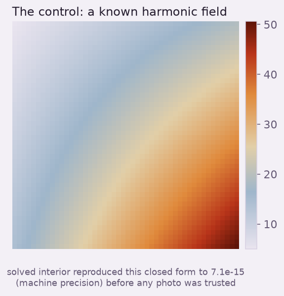
Before trusting a single healed pixel, we ran a control, because a converged solve that is quietly wrong is the failure mode that costs you. We pinned a known harmonic field on the boundary of a small test patch, left the interior free, and required the solver to reproduce that closed-form field in the interior. It did — to 7×10⁻¹⁵, machine precision. Only then did the image itself get solved. And the reconstruction has its own built-in check: because every healthy pixel is pinned to the true value, the reconstructed image reproduces the original exactly everywhere outside the damage, which confirms the pixel-to-node mapping is right and that the healed pixels really are the solver’s output.

A known harmonic field rendered as a thermal contour, used as the solver control. — The control that runs before any photo is trusted. A closed-form harmonic field is pinned on the boundary of a test patch and the solver must reproduce it in the interior — here to seven parts in ten thousand trillion. A heat solver that cannot reproduce a known harmonic field has no business filling a photograph.

The solved temperature field for one color channel, rendered as an incandescent contour, and a zoom on a healed scratch. — The solved steady-state temperature field for one color channel, drawn as a heat contour — and this field is the repaired channel. The Ansys solver computed a temperature at every one of the 65,536 nodes; across the damage (outlined) those temperatures are the harmonic fill. The zoom shows a healed scratch settling smoothly into its surroundings.

Does it actually heal?

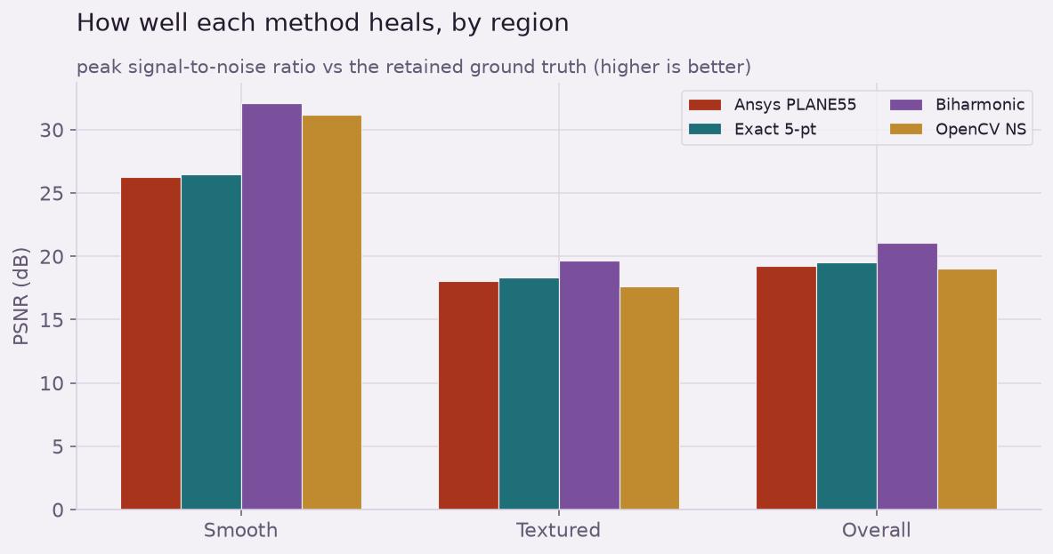
Because we kept the true original, we can put a number on the repair instead of eyeballing it. Overall, across all 2,689 damaged pixels, the Ansys reconstruction scores 19.2 dB PSNR (a root-mean-square error of about 28 gray levels on a 0–255 scale). That single number hides the real story, which is the split by region: 26.3 dB where the damage crosses a smooth area and only 18.0 dB where it crosses texture. The physics heals a scratch on the suit or the background so well you have to hunt for where it was, and it leaves a soft smear where a scratch crossed the flag or the hair. That is not a defect in the solve; it is the equation being honest about what diffusion can and cannot do.

The “same equation” claim gets its receipt here. We also solved the identical problem with the exact 5-point global harmonic solve — the discrete operator a diffusion healing brush relaxes to — and compared it to the Ansys PLANE55 result pixel by pixel. They agree to a mean of 1.16 gray levels (RMSE 2.0), with the largest single-pixel difference, about 19 levels, sitting on a hard edge where the two stencils weight neighbors differently. Same equation, two standard discretizations, a measured one-gray-level gap. That is what the equivalence between heat conduction and inpainting looks like when you actually check it.

Six panels: the damaged photo, the Ansys heat solve, the exact 5-point harmonic solve, biharmonic inpainting, OpenCV inpainting, and the ground truth, with PSNR labels. — The same damage healed five ways, against the true original. The Ansys PLANE55 heat solve (19.2 dB) and the exact 5-point harmonic fill (19.5 dB) are the pure diffusion answers and are nearly identical. Biharmonic inpainting (21.1 dB) is a higher-order relative that continues gradients better; OpenCV’s inpaint (19.0 dB) is what a real editor’s diffusion healing tool runs. All of them heal the smooth regions cleanly and blur the texture — the shared signature of diffusion.

Grouped bar chart of PSNR by region (smooth, textured, overall) for four healing methods. — How well each method heals, split by region. Every method scores far better on smooth damage than on textured damage — the gap between the left and middle groups is the whole point. The Ansys heat solve tracks the exact 5-point harmonic solve closely everywhere (the two diffusion answers), while the biharmonic and OpenCV fills edge ahead on smooth regions by using higher-order or more local diffusion.

Where the physics wins, and where it can’t

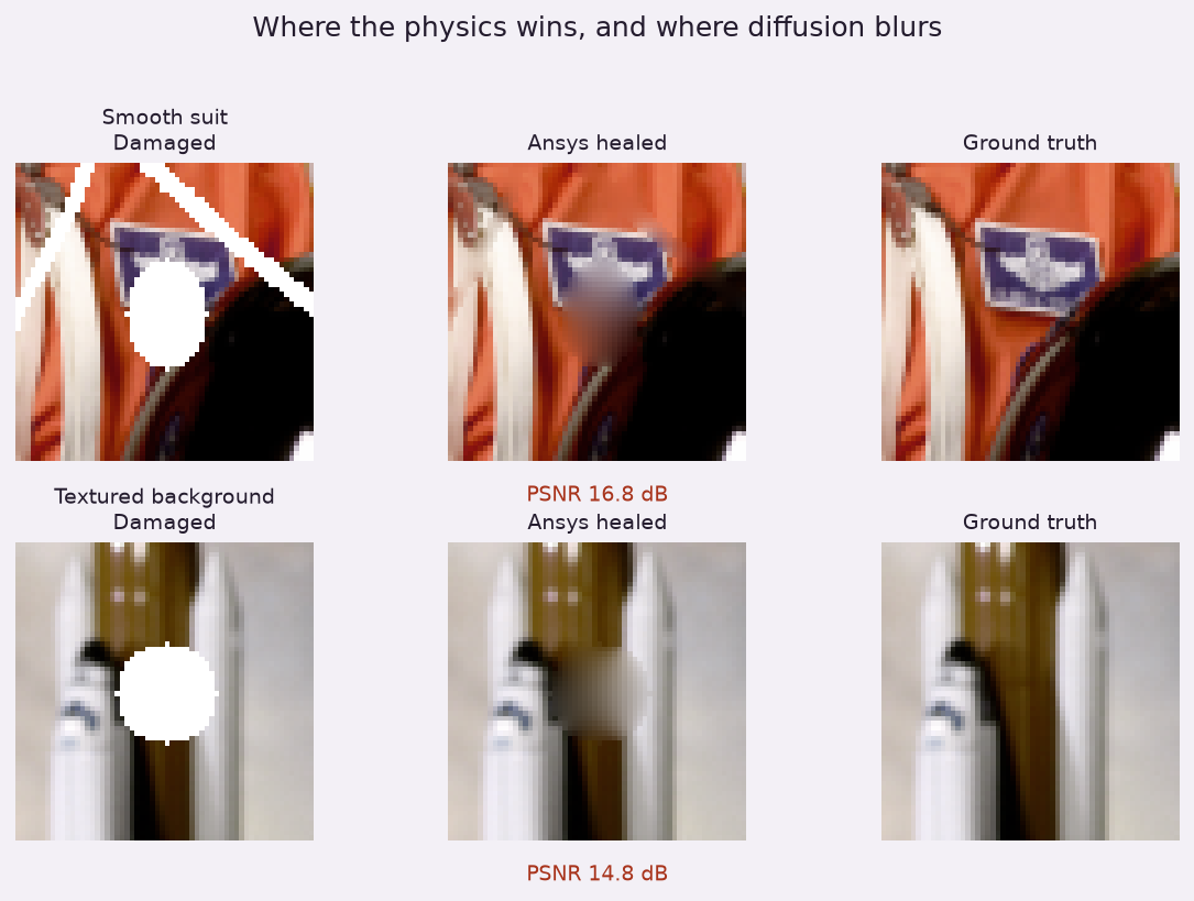
Line the two cases up and the boundary of the analogy is obvious. A blotch on the smooth orange suit heals to 16.8 dB and reads as clean at normal viewing size — the diffusion fill has nothing to reconstruct but a gentle gradient, and a gradient is exactly what harmonic functions are made of. A blotch of the same size over the textured, high-frequency background heals to only 14.8 dB and comes out as a soft, obvious smear, because there is no way for a smoothness-only rule to reinvent the fine structure that was there. The solver did not fail; it did precisely what ∇²T = 0 tells it to do.

Crops comparing a healed blotch on the smooth suit versus a healed blotch on the textured background. — Where diffusion wins and where it blurs. Top: a blotch on the smooth suit heals cleanly. Bottom: a blotch of the same size on the textured background comes back as a soft smear. This is the exact line between classical diffusion healing and modern content-aware fill — the latter copies real texture into the hole with a texture-synthesis algorithm (PatchMatch), a different method that beats diffusion precisely here.

Against a real photo editor

To make sure the physics equivalence is real and not a story we told ourselves, we healed the identical damage with a real editor’s diffusion tools: OpenCV’s inpaint, in both its Navier–Stokes and Fast-Marching modes — the diffusion algorithms that consumer healing brushes are built on. They scored 19.0 and 18.4 dB, the same ballpark as the Ansys solve, and they blur the texture in the same places. We also ran biharmonic inpainting (which solves ∇&sup4;u = 0, a higher-order cousin that continues gradients across the hole rather than just flattening them); it reached 21.1 dB overall and 32.1 dB on smooth regions, the best of the diffusion family and a fair picture of the ceiling this class of method can reach.

Two honest qualifications go with that comparison. OpenCV is a computer-vision library rather than a consumer app, but it runs the same diffusion mathematics a photo editor’s healing brush runs, so the comparison is like-for-like on the physics. And the consumer tools that clearly beat all of this on textured damage — content-aware fill and its kin — win not with better diffusion but with a different idea entirely: they synthesize texture by copying patches from elsewhere in the image. That is a genuinely separate algorithm, and it is exactly the part a heat solver was never going to do.

Honest scope. The repair is a genuine Ansys Mechanical steady-state thermal finite-element solve (PLANE55 elements, ∇²T = 0, unit conductivity), with every healthy pixel imposed as a fixed-temperature boundary condition and the recovered temperature field taken as the healed image; the solver was validated against a closed-form harmonic field to machine precision before any photo pixel was trusted, and the reconstruction reproduces the true image exactly outside the damage. What it is not: it is not content-aware fill or texture synthesis (PatchMatch), which is a different, non-physics algorithm — our equivalence and every number here are for classical diffusion healing only. Diffusion is smooth by construction, so it cannot rebuild texture or continue a sharp edge through a hole; the textured-region scores are honestly worse for that reason and are reported as they landed, not tuned. The damage is synthetic (added by us) so that a ground-truth PSNR/RMSE exists; a repair of unknown real damage has no such score. The three color channels are solved independently with no cross-channel coupling, and the model is a single steady (harmonic) solve — the higher-order biharmonic fill is shown as the named refinement, not modeled in Ansys. The image is public-domain NASA imagery; the numbers are what the converged solve and the retained original produce.

Have a field problem hiding inside something that doesn’t look like one? The same honest, end-to-end approach that turned a scratched photograph into a heat-conduction problem — recognizing the governing equation, building the right finite-element model, validating it against a known answer, and reporting exactly where it holds and where it doesn’t — is how we put real numbers on the physics your product actually runs on. That is innovation through insight.