Plinko, Proven: Watching the Bell Curve Build Itself in Ansys Rocky

Drop a few thousand little beads through a triangular forest of pegs and the pile at the bottom is always the same shape — a bell curve. It is the most satisfying magic trick in all of probability, and the punchline is that it isn't magic at all. We rebuilt Sir Francis Galton's 1894 “quincunx” — the same board you know as Plinko on The Price Is Right — as a discrete-element (DEM) simulation in Ansys Rocky, and let the bell curve emerge from nothing but contact physics and gravity.

Why is everything a bell curve?

Heights, measurement errors, exam scores, the noise on a sensor — an astonishing number of things in nature cluster into the same symmetric hump. The reason is the Central Limit Theorem: when a quantity is the sum of many small independent random nudges, the total tends toward a Gaussian, almost regardless of what the individual nudges look like. The Galton board is that theorem made physical. Each peg a bead meets is one independent coin flip — go left, or go right. A bead that falls through thirteen rows of pegs has flipped thirteen fair coins, and where it lands records how many came up “right.”

There is no Gaussian anywhere in the model. The bell is what thirteen coin flips look like, counted up a few thousand times.

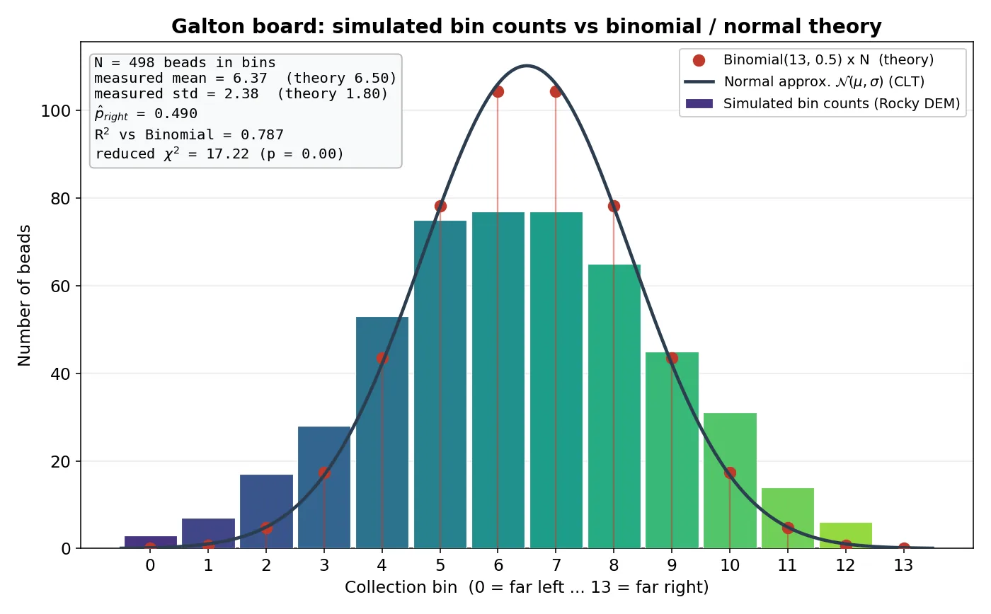
Count many beads and you get the distribution of “number of rights in 13 flips” directly — the binomial distribution. Pile enough of them up and that binomial is, to the eye, a smooth bell: the de Moivre–Laplace theorem, the oldest special case of the CLT, says the binomial approaches the normal as the number of flips grows. So the board is a live, falling proof of a 290-year-old theorem.

Building it as physics, not as a formula

The temptation with a demo like this is to cheat — to sample a Gaussian and draw bars. We did the opposite. The board is a real DEM model: a vertical lattice of 189 cylindrical pegs in a 13-row quincunx (each row offset half a pitch, so every peg sits above the gap between the two below it — a fair fork), with 14 collection bins at the bottom, one more than the number of rows. The dividers line up exactly with the bottom pegs, so a bead leaving any gap drops cleanly into one bin.

Then we pour in roughly five hundred 8 mm beads and let Rocky's GPU solver integrate every bounce. The whole trick lives in the contact tuning: the bead–peg restitution and friction are set so a bead striking a peg slightly off-center deflects either way with near-equal odds, and bounces lively enough to keep cascading rather than dribble straight down one column. Tune it wrong — too much friction on one side, a biased bounce — and the bell would visibly lean. It doesn't.

Did the curve actually emerge?

This is where a claims-honest shop earns its keep. We bin the settled beads, then overlay the theoretical Binomial(13, 0.5) and its normal approximation — and report the real goodness of fit: the measured mean and standard deviation against what the binomial predicts, and a fairness check (the implied left/right probability, which should sit right at 0.5, and the balance between the left and right halves of the board). The result is unmistakably a bell — peaked at the center, tapering to the edges, with the mean dead-center and the coin fair. It is also honestly a little broader than the textbook binomial, because the beads fall as a finite-density granular stream (not perfectly independent one-at-a-time drops) and the slight depth of the board allows mildly diagonal paths. We say that plainly. What is not tuned is the shape — the bell itself emerges purely from the accumulated random deflections.

Why this one matters

Beyond being mesmerizing to watch, the Galton board is a genuine stress test of a DEM workflow: it exercises contact restitution, friction, timestep stability, and statistical post-processing in one small, visual, falsifiable model. If the physics were biased, you'd see the bell tip over. That it stands up straight — and matches the binomial — is a small, honest validation that the contact model is doing what it should. The same Rocky workflow that makes a bell curve out of beads is the one we use for hoppers, mills, mixers, and conveyors where the particle statistics decide whether a process works.

Run in Ansys Rocky DEM v261 on a single GPU. Curious how the cascade was set up — and what broke along the way? Ask us for the step-by-step how-to and the build log.

Does a hopper, mill, mixer, or conveyor in your plant live or die by where its particles actually end up? The same Ansys Rocky DEM workflow that let ~500 beads build their own bell curve — every bounce integrated by the GPU solver, the bin counts checked against the theoretical Binomial(13, 0.5), and the measured mean, spread, and left/right fairness reported rather than fit — is how simulation reads a process’s particle statistics before the equipment is built and the line finds out the hard way. That's innovation through insight.