One Hull, Four Solvers: How a Boat Meets Water in Ansys AQWA, Rocky DEM, LS-DYNA ICFD, and Fluent VOF
“A boat in water” sounds like one simulation. It is really several — and which physics you reach for depends entirely on the question you are asking. Do you want the roll period of a tanker in a design sea state? The way a hull rides a shifting bed of solids? The shape of a free surface around a floating hull? Those are different governing equations and different Ansys solvers. So we floated the same boat through four of them, spanning three kinds of physics — Ansys AQWA (frequency-domain potential flow), Ansys Rocky (granular discrete-element), and the two free-surface CFD codes, Ansys LS-DYNA ICFD and Ansys Fluent VOF — and let each answer the part of the question it was built for. The honest comparison, including where each method stops, is the whole point.
| Solver | Physics | What the boat does | Best for |
|---|---|---|---|
| AQWA | Linear potential flow, frequency domain | Rocks — RAOs in a JONSWAP swell | Seakeeping, mooring, motions design |
| Rocky DEM | Discrete-element granular contact | Bobs on a “sea” of marbles | Solids handling, free-body-in-media |
| LS-DYNA ICFD | Incompressible Navier–Stokes, level set | Floats at its computed waterline | Fast / violent free surface, slamming |
| Fluent VOF | Incompressible Navier–Stokes, volume-of-fluid | Floats at its waterline (mass-conserving) | Sustained float, sloshing, fill / drain |
Act I — AQWA: the naval architect’s answer
Ask a naval architect how much a ship rolls and they will not run a transient CFD job — they will solve it frequency by frequency. AQWA treats the water as an inviscid potential flow and runs a diffraction/radiation analysis: it computes how the hull scatters incoming waves and how it radiates waves when it moves, giving the added mass, wave damping, and exciting force at every frequency. Feed those into the 6-DOF equation of motion,
−ω²(M + A(ω))·X + iωB(ω)·X + C·X = F(ω),
solve the complex linear system at each ω, and you get the Response Amplitude Operators — the transfer functions from wave height to heave, roll, and pitch. Multiply by a sea spectrum and you have the ship’s motion in a real seaway. We ran a 257 m VLCC crude tanker through exactly this pipeline, then rode it through a JONSWAP swell.
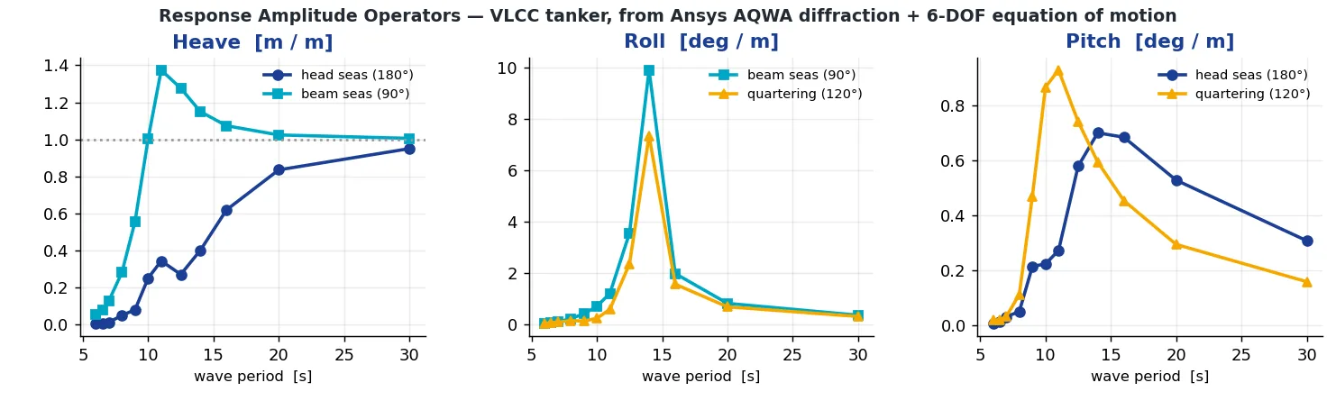
AQWA runs its traditional deck-and-solver workflow, so the entire study — writing the classic AQWA deck, launching the
solver, parsing the .LIS results into RAOs, and reconstructing the 6-DOF motion under a JONSWAP spectrum
— is Python driving that workflow end to end.
Act II — Rocky DEM: what if the sea were marbles?
Now change the question entirely. Instead of water, make the “sea” a bed of thousands of discrete particles, and ask how a free body rides it. That is a discrete-element problem, and Ansys Rocky solves it on the GPU — integrating the motion of every grain under gravity and resolving each grain-on-grain and grain-on-wall contact with a real force law. We dropped a boat hull onto ~3,400 twelve-millimeter “marbles” and shook the tank.
The engineering substance is real: every marble is a solved body, and the boat is genuinely free, pushed around by the granular bed. Driving it was its own exercise — the remote-control route wasn’t available on this machine, so the whole study runs in-process through Rocky’s own scripting host (build the project, fill the bed with a volumetric inlet, attach a free-body motion frame to the hull and a vibration frame to the tank, solve on the GPU).
Act III — The real fluid, two ways: LS-DYNA ICFD and Fluent VOF
Finally, the proper fluid — and here we did it twice, with the two different ways a CFD code tracks a free surface. LS-DYNA’s ICFD solver uses a level set; Ansys Fluent uses the volume-of-fluid (VOF) method. Both solve incompressible Navier–Stokes with real water and air, and both should float our box barge at the draft where buoyancy balances its 0.54 kg weight. So we built the same boat-in-a-tank in each and let it sit.
That last word is the whole point of running both. The level set is fast and elegant, but the single-fluid formulation is not mass-conserving over long times in a sealed tank — left alone, the surface slowly creeps. Fluent’s VOF method tracks the actual fraction of water in every cell, so it conserves mass and the waterline stays put. That is exactly the trade-off a free-surface analyst lives with: the level set is superb for fast, violent events (slamming, green water on a deck), while VOF is the tool for a sustained float, a slow slosh, or anything where the volume of water has to stay right deep into the run.
So which one should you actually use?
All four. That is the real lesson — they are not competitors, they are different questions:
- Design seakeeping → AQWA. Need roll/heave/pitch RAOs, mooring loads, operability across a scatter diagram? Potential flow gives you the whole frequency response in minutes, not the days a transient CFD sweep would cost. It is the industry default for a reason.
- A real free surface → CFD. Slamming, green water, sloshing, capsize, a wave breaking over a deck, or just a hull sitting at its true waterline — anything where the surface itself matters — needs the full Navier–Stokes treatment that linear potential-flow theory can’t represent. And within CFD, pick your free-surface method: the level set (LS-DYNA ICFD) is leanest for a fast, violent transient, while volume-of-fluid (Fluent) conserves mass for a sustained float or a slow slosh.
- Solids, not liquids → Rocky DEM. Bulk material handling, a body moving through grain, ballast, conveyors, mixers — the discrete-element world — is where the marble-sea coupling becomes a real engineering tool.
Have a floating structure, a sloshing tank, a slamming load, or a bulk-solids problem? Seakeeping in AQWA, free-surface CFD in Fluent and LS-DYNA, and discrete-element studies in Rocky are all core Rand Simulation work — and knowing which one your question actually needs is half the value. That’s innovation through insight.