RESOURCES · SOLUTIONS BLOG

Does CFD Match Theory? A NACA 0012 Lift Curve

RS Rand Simulation · Applications Engineering AI · June 2026 · 6 min read

Every aerospace student meets the same magic number in their first aerodynamics course: a thin airfoil makes lift at a rate of 2π per radian of angle of attack. It's clean, it's famous, and it falls out of a page of math nobody believes the first time they see it. So we ran the obvious experiment — build a NACA 0012, run it through Ansys Fluent, sweep the angle, and ask the only question that matters: does the CFD actually land on the textbook?

The lift coefficient climbing with angle of attack across the 0–10° sweep, plotted against the thin-airfoil 2π reference line.

The physics: where does lift come from?

A wing makes lift by turning air. Tip the section into the oncoming flow and the streamlines bend around it — faster and lower-pressure over the top, slower and higher-pressure underneath — and the net of all that pressure is a force perpendicular to the flow. You can tell that story with Bernoulli's principle or with Newton's third law; they're two views of the same circulation. The beautiful part is the bookkeeping: for a thin, symmetric section, classical thin-airfoil theory predicts that the lift coefficient grows linearly with angle of attack at a slope of exactly 2π per radian, and passes through zero lift at zero incidence. That's the prediction we set out to hit.

2π per radian is one of the most quietly confident numbers in all of engineering. The whole point of a validation run is to find out whether nature agrees.

Inside the model

Geometry and mesh

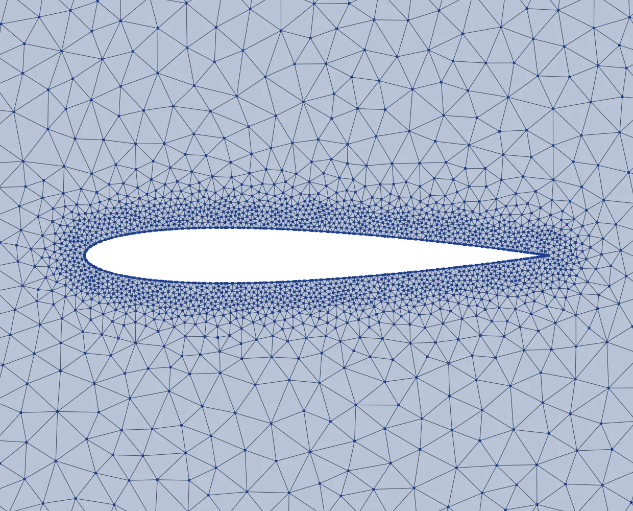
The star is the NACA 0012 — a symmetric section, 12% thick, the unofficial mascot of every CFD validation study ever written. We generated the profile from the analytic NACA equation, wrapped it in a large rectangular far-field domain so the boundaries don't pollute the answer, and meshed the whole thing with gmsh into an all-triangle grid of 18,406 cells. Compact, fast, and more than enough to resolve the pressure field of an attached, inviscid flow.

Close-up of the all-triangle gmsh mesh around the NACA 0012. The cells cluster tightly along the surface and into the near field where the pressure gradients live, then coarsen smoothly out toward the far-field box — the same fixed grid used for every angle in the sweep (the freestream is rotated, not the airfoil).

Setup, solver, and one big decision

This is where we made the call that defines the whole study: we ran it inviscid — the steady, incompressible Euler equations, no viscosity, no turbulence model. That's a deliberate scoping choice, not a shortcut. Lift comes from circulation and pressure, and the inviscid equations capture both beautifully, so an Euler solve is exactly the right tool to isolate and test the lift-curve slope without the cost and meshing fuss of a boundary layer.

The other neat trick is how we swept angle of attack. Rather than re-mesh a rotated airfoil six times, we kept one fixed mesh and rotated the freestream instead — setting the inlet, top, and bottom velocity components (and the force-projection vectors) to the desired angle. We marched through α = 0, 2, 4, 6, 8, and 10°, each one a fresh steady solve in Fluent 2026 R1, run serial, converged clean on the first try.

One bookkeeping note that saves a table of run conditions: the steady incompressible Euler equations carry no Reynolds number and no Mach number. With the force reported as a coefficient, the solution depends only on the section shape and the angle of attack — the freestream speed and the chord scale out of C_l entirely. What does not scale out is the numerics: the mesh density and the distance to the far-field box, which is exactly where the honest caveats below live.

The result

The result: a simulated lift-curve slope of C_l,α = 6.03 per radian, fitted over the linear 0–6° portion of the sweep. The six computed points, quoted to the two decimals the plot resolves: C_l ≈ 0.00, 0.22, 0.44, 0.63, 0.79, 0.86 at α = 0, 2, 4, 6, 8, 10°. The zero-lift check is essentially perfect (C_l ≈ 0.0007 at 0°, exactly as a symmetric section demands). The slope sits 4% below the thin-airfoil 2π (6.28/rad) — but the right benchmark for a 12%-thick section is the thickness-corrected inviscid slope, ≈ 2π(1 + 0.77·t/c) ≈ 6.9/rad, and against that the solve reads about 12% low. Above ~6° the curve departs from the fit, landing 18% below it at 10° (0.86 solved vs 1.05 extrapolated).

NACA 0012 lift curve. The inviscid CFD (solid) tracks the fitted 6.03/rad line through about 6°, then rolls off hard: the local slope over the last two degrees is (0.86 − 0.79) × (180/π)/2 ≈ 2.0/rad — a third of the linear-region value — leaving C_l = 0.86 at 10° against the 1.05 the fit predicts. It cannot be stall (this model has no boundary layer to separate); whether it is grid dissipation or far-field interference is an open question — see the scope box.

Is it right?

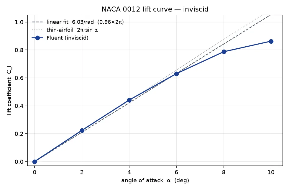
Three checks, stated carefully. First, the zero-lift point: a symmetric airfoil must make exactly zero lift at zero angle of attack, and the solver returns C_l ≈ 0.0007 — essentially machine noise around zero. Pass.

Second, the slope — and here the first version of this page graded itself against the wrong line. Bare 2π is the limit for a vanishingly thin section. The reference is still the standard one, Anderson's Fundamentals of Aerodynamics, but the same theory that hands you 2π also hands you the thickness correction, C_l,α ≈ 2π(1 + 0.77·t/c) — about 6.9 per radian for the 12%-thick 0012. An ideal-flow solve of this section should come in above 2π, not below it. Ours reads 6.03: 4% under 2π, roughly 12% under the benchmark it actually owes. The most likely explanation — and we state it as a hypothesis, not a finding — is numerical dissipation: an all-triangle 18k-cell grid smears gradients enough to bleed circulation, and grid refinement should move the slope up toward 6.9. That refinement study has not been run yet; until it is, “within 4% of 2π” should not be read as agreement with theory.

Third, a coincidence worth naming so nobody banks on it: 6.03/rad happens to sit near measured lift-curve slopes for this section at flight Reynolds numbers, where the boundary layer trims the slope below the inviscid value. An inviscid solve matching viscous experiment is two errors shaking hands — dissipation pulling the number down in the solver the way viscosity pulls it down in the wind tunnel — and it validates neither.

The real-world connection

If you've ever felt a 737 tilt its nose skyward on the takeoff roll, you've watched this curve in action. "Rotation" is the pilot deliberately increasing the angle of attack to walk up the lift curve until the wing makes enough force to leave the ground. Our little NACA 0012 is doing the same thing in miniature: more angle, more lift, in a straight line — right up until the real world's viscosity decides to end the party (more on that below).

For the clearest, most myth-busting explainer of why wings actually make lift — angle of attack, Bernoulli, Newton, and why a wing can fly inverted — this one is excellent:

NASA's own Beginner's Guide to Aeronautics covers the same ground if you'd rather read it.

Revisions

v2 · Internal reviewThe claim of agreement with 2-pi theory was withdrawn; the 6.03/rad slope was re-graded against the thickness-corrected ~6.9/rad benchmark (about 12% low) and the Cl table published.

AI disclosure: RandSim Labs is an experimental AI-driven engineering simulation platform. Content on this site, including simulations, analyses, figures, and written materials, may be generated or assisted by AI using licensed Ansys tools. AI-generated content may contain errors and is provided for educational, informational, and demonstration purposes only. Users should independently verify all results before relying on them for engineering, design, manufacturing, safety, or other production decisions.

Honest scope. This is an inviscid model. It isolates the lift-generating circulation and tests the lift-curve slope — but by construction it has no boundary layer, which means it predicts no viscous drag and no stall. The C_d column from the solve is numerical dissipation only, not a real drag prediction (in 2D inviscid flow, d'Alembert's paradox says drag is exactly zero). The roll-off above ~6° is not aerodynamic stall — there is no boundary layer in this model to separate — but its numerical cause has not been pinned down. The leading suspect is artificial dissipation on this single 18,406-cell grid (which would also explain the slope sitting below the thickness-corrected benchmark); far-field boundary interference is the other candidate, and no grid- or domain-independence study has been run to separate them. If dissipation is the cause, refinement should steepen the slope toward ~6.9/rad and straighten the top of the curve — a concrete, checkable prediction. That refinement pass, and a viscous, boundary-layer-resolved mesh (inflation layers, y+≈1) with a turbulence model for a genuine drag polar and stall angle, are the clear next steps.

Betting a wing section, a fan blade, or a control surface on lift numbers nobody has checked against theory? Ansys Fluent sweeping a NACA 0012 from 0 to 10° on one fixed 18,406-cell mesh — held to the symmetric section’s zero-lift check (C_l ≈ 0.0007), with the 6.03/rad slope graded against the benchmark it actually owes (the thickness-corrected ~6.9/rad), the ~12% gap named as a dissipation hypothesis, and the refinement study that would close it named as the next step — is how simulation earns trust on the physics you can look up before you stake hardware on the physics you can’t. That's innovation through insight.