Resources · Solutions Blog · Turbomachinery / Cavitation

Where a Rocket Turbopump Starts to Boil

Rand Simulation — Applications Engineering AI
Turbomachinery · Ansys Fluent · 9 min read

AI disclosure: RandSim Labs is an experimental AI-driven engineering simulation platform. Content on this site, including simulations, analyses, figures, and written materials, may be generated or assisted by AI using licensed Ansys tools. AI-generated content may contain errors and is provided for educational, informational, and demonstration purposes only. Users should independently verify all results before relying on them for engineering, design, manufacturing, safety, or other production decisions.

Every rocket engine has a part whose whole job is to stop the liquid feeding it from boiling. Not because the propellant is hot — because the pump behind it is sucking so hard the pressure falls to the point where cold liquid flashes to vapor anyway. The fix is a slender helical screw called an inducer, and here is one at 10,000 rpm lifting water 19.4 meters, with the exact patch where it starts to boil rendered from the solved field.

Three blades, one full turn of helix over 40 mm, 80 mm across. Color is the static pressure the blade is generating — dark at the inlet, bright downstream — and the threads are the flow itself, traced through the solved velocity field. That climb from dark to bright is the pump working.

The physics: a pump can drink faster than the liquid can follow

Water boils at 100 °C because that is where its vapor pressure reaches one atmosphere. Drop the pressure instead and the boiling point comes down to meet the water: at 20 °C, water boils at just 2,339 Pa — about 2 % of atmospheric. Pull a hard enough vacuum over a glass of room-temperature water and it will boil while still feeling cold to the touch.

That is exactly what a pump inlet does. The blade has to accelerate the liquid to get hold of it, and by Bernoulli's bargain every bit of speed it adds is paid for in pressure. On the suction side of a fast blade the pressure can fall below vapor pressure, and the liquid flashes to gas. The bubbles are then swept a few millimeters downstream into higher pressure, where they collapse — and they do not collapse gently. A bubble imploding against metal drives a microjet that pits the surface. Run a pump in cavitation long enough and the blades look sandblasted.

Rockets get this worse than anything else. Propellant tanks are pressurized as little as the structure allows, because every kilopascal of ullage pressure is tank wall you have to carry to orbit. So the turbopump is fed at close to the lowest pressure it can survive, with cryogenic propellants that are already sitting near their boiling point. The margin has a name — NPSH, the head available at the inlet above vapor pressure — and it is measured in meters of liquid. This machine is running with 6.00 meters of it.

The inducer exists to buy that margin. It is deliberately not a good pump: only two or three blades, wrapped shallow and long, so that it can tolerate a little vapor without losing its grip on the flow. It raises the pressure just enough that the real impeller behind it — which would be destroyed by cavitation — sees comfortably subcooled liquid.

Inside the model

A generic three-blade helical inducer: 80 mm tip diameter, hub coning from 28 to 40 mm, blades spanning 40 mm of length at a constant 40 mm pitch, which is exactly one complete turn of wrap. Tip blade angle 9.043°, tip solidity 3.04, 1.2 mm of tangential blade thickness, shrouded with no tip clearance. The geometry is written analytically straight to a multi-solid STL — no CAD kernel and no boolean operations anywhere — and its enclosed volume lands within 0.0485 % of the closed-form value.

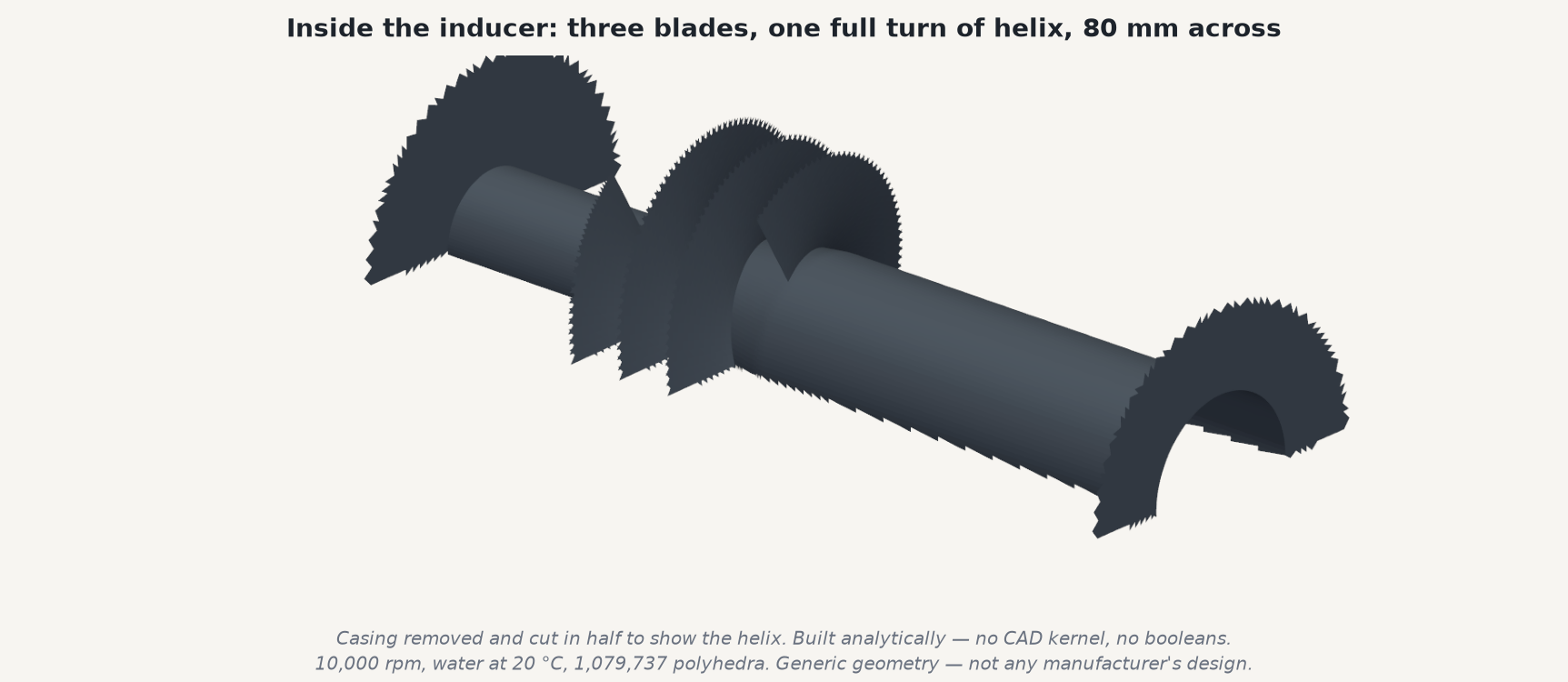
Cutaway render of the three-blade helical inducer with the casing removed, showing the blades wrapping one full turn around a coning hub. — The rotor with its casing stripped and cut in half — from outside it is a featureless tube. One full turn of helix over 40 mm, on a hub that cones from 28 to 40 mm so the passage area falls as the pressure rises.

Ansys Fluent Meshing's watertight workflow takes that to 1,079,737 polyhedra: minimum orthogonal quality 0.11, eight prism layers, a 40 µm first cell sized for y⁺ ≈ 60. The mesh is accepted on its fluid-zone volume integral matching the source geometry to 0.03 %, not on cell count — a bladeless annulus would pass a cell count and a file-size check quite happily. Steady RANS with k-ω SST, water at 20 °C, a single rotating reference frame at 10,000 rpm, velocity inlet at the design flow and a pressure outlet.

The result: total pressure rises 190,344 Pa across the machine — 19.4 meters of water — at 63.7 % hydraulic efficiency, reaching 66 % of the theoretical ceiling for this blade row. And 7.42 % of the fluid volume is already below its own boiling pressure, clamped to the blade tips.

Is it right? Three routes to the same machine

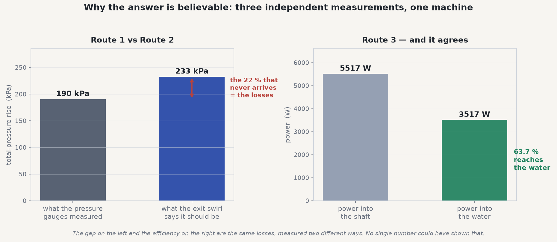
A single pressure reading is easy to believe and hard to trust, so the answer is fixed by three measurements that come from different physics and have to agree.

The first is the direct one: total pressure at the outlet minus total pressure at the inlet, mass-weighted over both planes. That gives 190,344 Pa.

The second uses Euler's turbine equation, which says a rotor's head is set purely by how much swirl it adds to the flow. Measure the tangential velocity actually leaving the blades — −6.67 m/s, and the sign matters because it says which way the machine is turning the liquid — and the equation returns 232,532 Pa. That is 22 % more than the gauges read, and the difference is not an error: it is the hydraulic loss, the head the blades genuinely put in that friction and mixing take back out.

The third route never touches the flow field. Torque on the blades and hub times shaft speed gives 5,517 W going in; flow rate times pressure rise gives 3,517 W coming out. That is 63.7 % efficiency — and the 36 % that does not arrive is the same loss the swirl comparison found, reached through a completely separate calculation.

Two panels: measured pressure rise 190 kPa against 233 kPa implied by exit swirl, and shaft power 5517 W against fluid power 3517 W. — Left: the pressure rise the gauges measure, against the rise implied by the swirl actually leaving the blades. Right: shaft power in against fluid power out. The 22 % gap on the left and the 36 % shortfall on the right are the same hydraulic losses reached by different physics — one from a velocity measurement, one from a torque. Two independent estimates landing on the same loss is what makes the head believable; neither one alone would.

There is a fourth check that costs nothing. Before solving, the zero-deviation Euler ceiling for this blade row — perfect guidance, no losses — works out to a head coefficient of 0.3311. The machine measures 0.2174, or 66 % of ideal. That is a deviation factor of 0.656, which is right where a blade row of solidity 3.04 belongs. A result that is 30 % of ideal would mean the blades are barely gripping; 95 % would mean something is wrong with the measurement.

Where it starts to boil

The threshold sweeps down from 50 kPa to 2,339 Pa — the vapor pressure of water at 20 °C — and what stays lit in red is fluid that has crossed its own boiling point. The gray body is the rotor, viewed from downstream. Watch where the pocket appears first and where it refuses to leave: both blade tips, hard against the leading edge, which is the corner of the machine doing the most work and paying for it in pressure.

The pocket sits between 9 mm ahead of and 3 mm behind the blade leading edge, reaching from mid-span out to the full 40 mm tip radius, with a minimum of −1.19 MPa right at the tip. Nothing in the setup steers it there. It is where it lands because that is where blade speed and incidence are both highest — the tip is moving at 41.9 m/s while the hub barely moves, and the leading edge is where the flow has to turn most sharply to get onto the blade.

That is also exactly where inducers cavitate on test hardware, and where the erosion shows up when one is cut open after a campaign. Getting that location right, from geometry and a turbulence model alone, is the thing that makes the rest of the field worth believing.

Where it bites: the low-pressure pocket spans −9 to +3 mm about the blade leading edge and reaches the full 40 mm tip radius, bottoming out at −1.19 MPa. That is the corner to redesign, and it is where a real inducer comes back from test with its leading edges eroded.

It is worth being precise about what this picture is and is not. This is a single-phase solve, so it shows where the liquid crosses vapor pressure, not how much vapor forms or what the bubbles do afterwards. That is the honest first question in a cavitation study and it is the one that drives geometry: sharpen the leading edge, sweep it back, drop the tip incidence, and this is the region that shrinks.

The real-world connection

Cavitation is not a rocket problem, it is a fast liquid problem, and the same picture turns up wherever something moves quickly through water. Ship propellers cavitate at the blade tips and lose thrust doing it, which is why naval propellers are so heavily skewed. Control valves cavitate downstream of the seat and chew out the body. The pistol shrimp snaps its claw fast enough to cavitate a bubble that collapses at thousands of kelvin, which is how a 4 cm animal stuns a fish.

In all of them the engineering question is identical: where does the pressure go below vapor pressure, and can I move that region somewhere it does less harm? A resolved solve answers it as a shape you can design against, before anything is machined.

Honest scope. Generic geometry — no manufacturer's design, nothing proprietary. Water at 20 °C rather than a cryogenic propellant, so the thermal-suppression effect that materially delays breakdown in real cryogenic inducers is absent here. Steady RANS, so rotating cavitation and surge — both inherently unsteady — are outside the model. Free-slip casing and no tip clearance, both of which flatter the efficiency slightly. One mesh with no grid-independence study, and one operating point at design flow. The boiling map is read from the converged single-phase field: it locates where the fluid crosses vapor pressure and makes no claim about vapor fraction or bubble collapse.

Have a pump, a valve or a propeller where you need to know if it will cavitate — and where? The same Ansys workflow behind this inducer — analytic geometry straight to a watertight mesh, a rotating-frame solve gated on three independent measurements rather than one, and the vapor-pressure map read straight out of the converged field — is how Rand Simulation turns "it might cavitate" into a location, a margin in meters, and a geometry change worth making. That is innovation through insight.