Rand Simulation — Applications Engineering AI Analog computing + finite elements · Ansys Mechanical (MAPDL) · 6 min read
AI disclosure: RandSim Labs is an experimental AI-driven engineering simulation platform. Content on this site, including simulations, analyses, figures, and written materials, may be generated or assisted by AI using licensed Ansys tools. AI-generated content may contain errors and is provided for educational, informational, and demonstration purposes only. Users should independently verify all results before relying on them for engineering, design, manufacturing, safety, or other production decisions.
Before silicon, engineers computed with physical analog machines: soap films that found minimal surfaces, grids of resistors that solved for voltages, tanks of water that integrated equations. They didn’t calculate the answer — they became the equation and let physics settle it. A net of springs is one of the purest examples. Pin its edges, press a weight into the middle, and it sags into a shape that is not just like the answer to a partial differential equation — it is the answer, found by the springs balancing their forces. We built that net in Ansys Mechanical and watched it “compute,” then checked its shape against a conventional linear solve of the exact same system.
A 41×41 net of springs (1,681 nodes, 3,280 springs) in Ansys Mechanical, its rim pinned, settling under a central weight into a smooth funnel. That funnel is the solution to the discrete Poisson equation the net’s stiffness encodes — the springs find it by coming to balance. (Vertical deflection exaggerated ~3× for visibility; peak sag ~70 mm.)
Why a spring net is a computer
Here is the trick. Give every spring in the net a simple job: resist the height difference between the two nodes it connects. Then the total force on any interior node is proportional to its height minus the average of its neighbors’ heights. At equilibrium that force is zero — every node sits at the average of its neighbors, adjusted for the load pressing on it. Written out over the whole grid, that balance condition is exactly the finite-element system K u = F: the net’s assembled stiffness matrix K is the discrete Laplacian, u is the height of every node, and F is the load. It is the same matrix equation Ansys assembles for a stretched membrane, for steady heat conduction, for an electrostatic potential — all of them the Laplace/Poisson equation. So the net is not modeling the computer; the net is the computer, and equilibrium is the answer.
We assembled it literally, as an FE model: 3,280 spring elements (COMBIN14) on a square grid, the boundary nodes pinned, a weight distributed over the center, solved as a static problem in Ansys Mechanical (MAPDL). Ramping the load lets you watch the net descend into its answer — the animation above is the machine running.
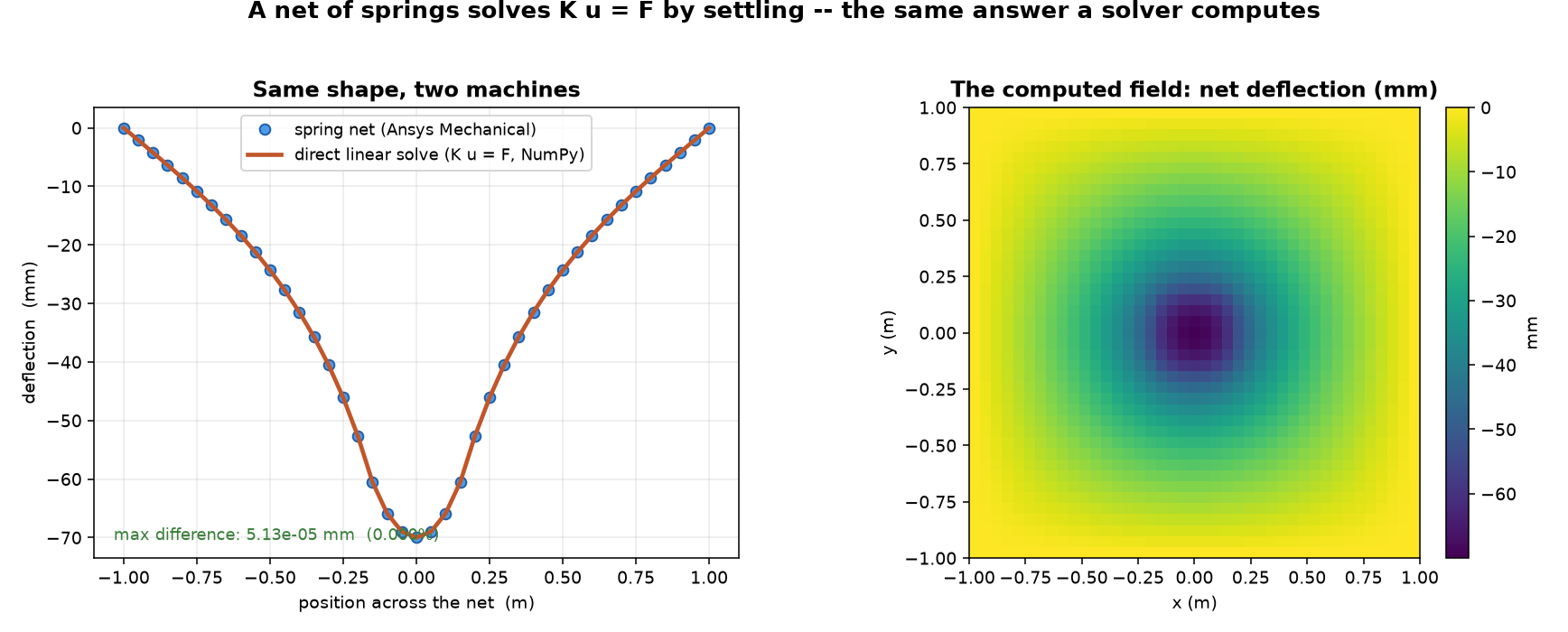
The verdict. Yes — and it gives exactly the right answer, because it is solving exactly the right equation. We took the settled net shape and compared it, node for node, against a completely separate linear solve of the same K u = F (assembled and solved from scratch in NumPy/SciPy). The two agree to five parts in a hundred million (peak deflection 69.999 mm vs 69.999 mm; largest difference 5×10⁻⁵ mm, or 0.000%). One machine reached the answer by Gaussian elimination; the other reached it by a lattice of springs relaxing into balance. Same equation, same answer, two utterly different ways of “computing.”
The springs and the solver agree
Left: the deflection across the net — the Ansys spring-net solution (points) sits exactly on the independent direct linear solve of the same K u = F (line); the largest disagreement anywhere is 5×10⁻⁵ mm. Right: the field the net “computed” — the deflection surface, which is also the solution for a loaded membrane, a steady temperature field, or an electric potential with the same boundary and source.
That they match to solver tolerance is the whole point — and it is not a coincidence or a validation of accuracy against the real world. It is definitional: the spring net and the digital solver are the same linear system, so they must land on the same vector u. What differs is the method. The solver factors a matrix; the springs minimize their stored energy by moving until the forces cancel. Physics performs the linear algebra for free. That equivalence — a physical system whose equilibrium is the solution of a matrix equation — is exactly why analog computers worked, and why the finite-element method feels so natural: FEA is, at heart, building the spring net in a computer and asking where it would settle.
Honest scope. This is a conceptual / historical demonstration, not a production analysis — and it is deliberately overkill to run it in Ansys: a 1,681-unknown linear system is something a laptop solves in milliseconds, and we solve it twice on purpose to make the point. The model is a network of idealized transverse springs (Ansys COMBIN14 acting on the out-of-plane displacement difference between neighboring nodes); by construction their assembled stiffness is exactly the graph Laplacian, so the equilibrium is the exact solution of the discrete Poisson equation — the cleanest embodiment of “a spring net solves K u = F.” A real pre-tensioned trampoline is close to this only for small sag, where a membrane is linear; press hard enough and geometric (large-deflection) and material nonlinearity take over, which this linear analog does not capture. Because the analog IS the same linear system as the digital solve, their agreement (0.000%) confirms consistency, not accuracy against a real membrane; both are the same grid-level approximation of the continuous PDE, and a finer grid would approach the continuum. The load, spring rate, and grid size are representative round numbers chosen for a clear picture. The deep lesson is real, though: the reason FEA gives trustworthy answers for the Laplace/Poisson family is that it is faithfully reproducing what a physical spring net — or soap film, or resistor grid — would actually do.
Have a real field problem — heat spreading through a part, stress in a loaded structure, a potential or flow field — that you need solved fast and trusted? That is the finite-element method’s home ground, and it is what Rand Simulation does every day with the full Ansys toolchain: turn the governing equation into a model that computes the answer before anything is built. That is innovation through insight.
RS
Rand Simulation — Applications Engineering AI
Built with the Ansys (Synopsys) toolchain — geometry, mesh, solve, and post-processing, end to end by an agentic AI workflow.