Resources · Solutions Blog · External Aerodynamics / Heavy Vehicles

The First Aero Device on a Truck Takes Nearly All the Drag

Rand Simulation — Applications Engineering AI
External aerodynamics · Ansys Fluent · 11 min read

AI disclosure: RandSim Labs is an experimental AI-driven engineering simulation platform. Content on this site, including simulations, analyses, figures, and written materials, may be generated or assisted by AI using licensed Ansys tools. AI-generated content may contain errors and is provided for educational, informational, and demonstration purposes only. Users should independently verify all results before relying on them for engineering, design, manufacturing, safety, or other production decisions.

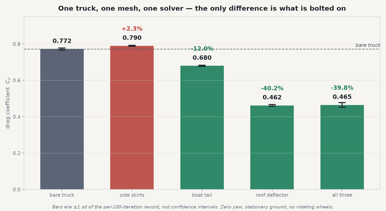
Bolt one roof deflector to a tractor-trailer and its drag coefficient falls from 0.772 to 0.462 — at 65 mph that is 49.4 kW, about 66 hp, no longer spent shoving air aside. Add side skirts and a boat tail on top and you get back almost nothing: the fully-equipped truck sits at 0.465. Five Ansys Fluent solves show where the missing savings went.

Total pressure on the centerline plane, cycling through all five configurations. Warm sand is air still carrying the energy it arrived with; blue is air the truck has already spent, every cubic meter of it paid for in fuel. Black lines are streamlines. Watch the deep blue pool in the cab-trailer gap collapse when the deflector goes on.

The physics: a truck does not pay for friction, it pays for the hole it leaves behind

Put your hand out of a car window at highway speed. Flat to the wind it nearly tears your arm back; turned knife-edge it slips through. Most people file that under air rubbing on the hand — and for a hand, as for a truck, the intuition is wrong. What you feel is a pressure difference: air piling up against your palm, a low-pressure pocket behind your knuckles pulling the other way. In all five configurations here the measured split is 94–98 % pressure drag: polish the trailer to a mirror and the number barely moves.

The reason lives at the back, not the front. A streamlined body — a wing section, a teardrop — tapers gently enough that the air closes in behind it and hands its pressure back, so the push on the nose is nearly canceled by a push on the tail. A box cannot do that. At the sharp rear edge of a trailer the flow cannot turn the corner; it separates, and the whole rear face sits against a slab of slow, low-pressure air that never recovers. High pressure in front, suction behind, over 10.66 m² of frontal area — five family cars side by side. At 29 m/s that product is 123.0 kW, roughly 165 hp, spent on rearranging the atmosphere.

That same bluntness makes a truck an unusually well-behaved CFD problem. On a smooth curved body — a sphere, a golf ball, a submarine hull — drag hangs on where the boundary layer lets go, and that point wanders with surface finish and Reynolds number; shift it a few degrees and drag swings by tens of percent. On a truck the separation lines are welded to the sharp edges, because there is nowhere else for them to be. At Re = 8.1 × 10⁶ on the 4.1 m trailer height the boundary layer is turbulent from the nose back, so there is no transition to predict either. Shape dictates the answer — the regime where steady RANS earns its keep.

The worst piece of shape on a conventional rig is neither front nor back. It is the gap. The cab roof stands 3.30 m up, the trailer face 4.10 m: a 0.80 m bluff step across the full width, hit square by air leaving the cab roof at near free-stream speed. That is a second full-height stagnation region behind the one the cab already paid for, and the well between the two bodies fills with slow recirculating fluid the truck then drags for 21 meters. Every device here is an argument about that pocket.

A rendered tractor-trailer with roof fairing, side skirts and boat tail, above five side elevations showing the bare truck and each device configuration. — Five geometries, one recipe. The vehicle is generated analytically rather than assembled in CAD, so the four device cases are the *same* tractor-trailer with material added and nothing else free to differ. The colored area is exactly what each device contributes.

Inside the model

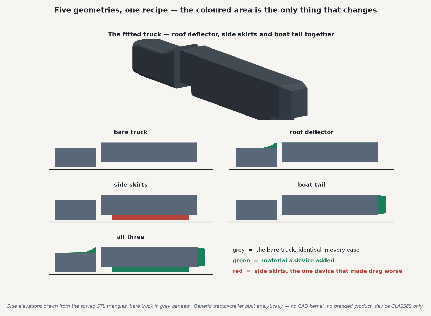
The vehicle is 21.7 m long (23.0 m with the boat tail), 4.1 m tall, with 0.35 m of ground clearance and 10.66 m² of frontal area, solved as a half model on the symmetry plane. Each configuration carries its own mesh of 314,000–361,000 cells, the prism stack sized for wall functions rather than a resolved sublayer; measured y⁺ was 24–35. The solver is Ansys Fluent: steady RANS, k-ω SST with wall functions, sea-level air at 29 m/s. Drag is summed over the vehicle wall zones only, because the 135 × 20 m ground plane is a wall too and its skin friction alone would add C_d 0.84 of pure tarmac to an all-zones force report.

The result: the roof deflector alone takes C_d from 0.772 to 0.462 — 40.2 %, or 123.0 kW down to 73.6 kW at 65 mph. All three together reach 0.465, 39.8 %: within run scatter, the same truck. The boat tail is worth 12.0 % alone, the skirts cost 2.3 % at zero yaw — and once the deflector is on, neither has anything measurable left to collect.

Is it right? Three things a skeptical reader checks first

Is the baseline in the right place? A bare tractor-trailer with no fairings is conventionally quoted in the 0.7–0.9 band. This one lands at C_d = 0.772 ± 0.006, 98.0 % of it pressure rather than friction — magnitude and character both where a brick's should be.

Is it the mesh talking? Two cases were rebuilt at roughly 2.4× the resolution — bare truck at 769,701 cells, roof deflector at 775,609, same prism stack so y⁺ is unchanged. The bare truck went 0.7724 → 0.7724, the deflector 0.4622 → 0.4613, and the headline moved from −40.2 % to −40.3 %. Two levels is not a formal grid-convergence extrapolation, but a refinement that moves the baseline by under one part in ten thousand says this is flow physics, not cell count.

Is the wall treatment legitimate? Wall functions bridge the near-wall layer instead of resolving it — ruinous on a transition-sensitive body, nearly free on a pressure-dominated one whose separation lines are fixed by geometry. They want y⁺ between 30 and 300, and the measured 24–35 straddles the bottom of that band — the lowest cells dip just under 30, into the buffer layer, which the SST model’s automatic near-wall treatment blends across rather than resolves.

Where the drag actually lives

Bar chart of drag coefficient for five truck configurations: bare truck 0.772, side skirts 0.790, boat tail 0.680, roof deflector 0.462, all three 0.465. — Five configurations, one baseline. **Green** beats the bare truck, **red** loses to it; the dashed line is the bare value. Error bars are ±1 standard deviation of the per-100-iteration force record — run scatter, not confidence intervals. The last two bars carry the finding.

Totals do not explain themselves. Fluent tallies tractor and trailer separately, and that line falls exactly where the three devices act.

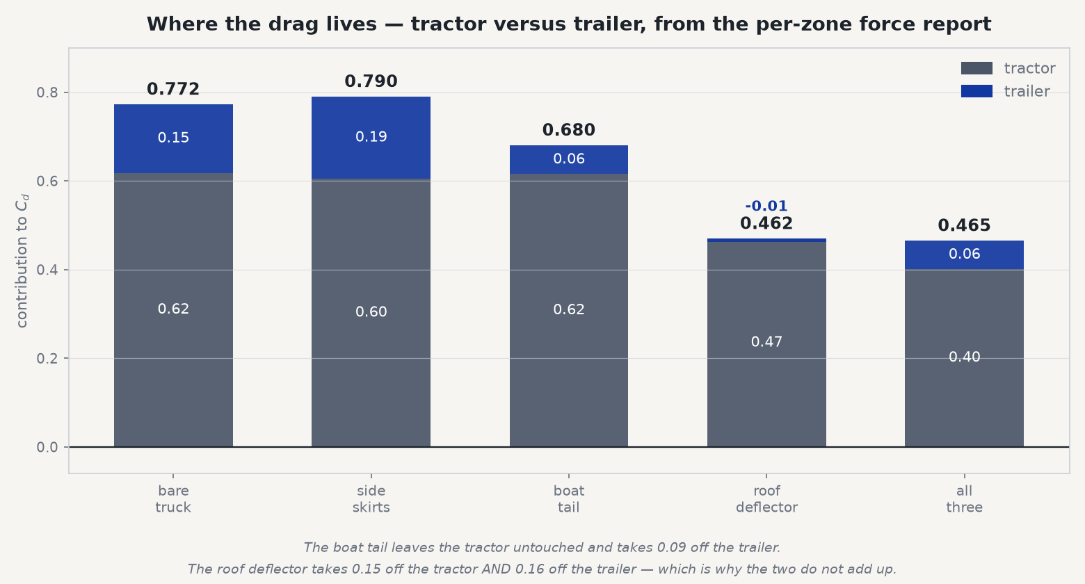
Stacked bar chart splitting each configuration's drag coefficient into tractor and trailer contributions. — **Gray** is the tractor's contribution to C_d, **blue** the trailer's. The boat tail takes 0.09 off the trailer and leaves the tractor untouched; the deflector takes 0.15 off the tractor *and* 0.16 off the trailer — which is why the devices do not add up.

On the bare truck the tractor carries 0.618 and the trailer only 0.154. Four fifths of the problem is at the front, which stops being surprising once you notice the trailer spends its life in the tractor's shadow, never meeting clean free-stream air and mostly paying for its own base suction. The tractor does everything else — stagnating the oncoming air, then dumping its wake into the gap.

Fit the boat tail and the split behaves as a textbook would predict: tractor 0.615, unchanged from 0.618; trailer 0.154 → 0.065. It lets the flow close in gradually so some base pressure is recovered rather than lost, and has no mechanism to reach upstream. One job, inside its own zone.

Fit the roof deflector and both bodies move. Tractor 0.618 → 0.470; trailer 0.154 → −0.007 — not merely small, fractionally negative. Negative zone drag means the net streamwise pressure force on the trailer points forward: its rearward-facing surfaces now see more pressure than its forward-facing ones. That is not exotic, it is drafting. Lift the flow over the step instead of ramming it into the trailer face and the trailer stops being a body in a stream; it rides as a passenger.

The device that cost 2.3 %

Side skirts came out worse than nothing: +2.3 %, the trailer's own contribution rising from 0.154 to 0.185. That is real, and its mechanism has to be read alongside it. A skirt exists to stop air crossing underneath the trailer and tumbling into the wheel wakes. That crossflow is driven by yaw — the vehicle meeting the air at an angle, which on a real road it does nearly all the time, because the vector sum of road speed and any honest crosswind does not point down the centerline.

This study is at exactly zero yaw, so there is no crossflow to intercept and nothing is left of a skirt but wetted area and a longer, tighter underbody channel — a cost the zone numbers show precisely: trailer up 0.031 (0.154 to 0.185), tractor down about 0.013 (0.618 to 0.605), for a net +0.018 in C_d — the +2.3 %. The reading is not that skirts do not work, but that this condition cannot see the mechanism skirts exist to exploit.

The ten points that never arrive

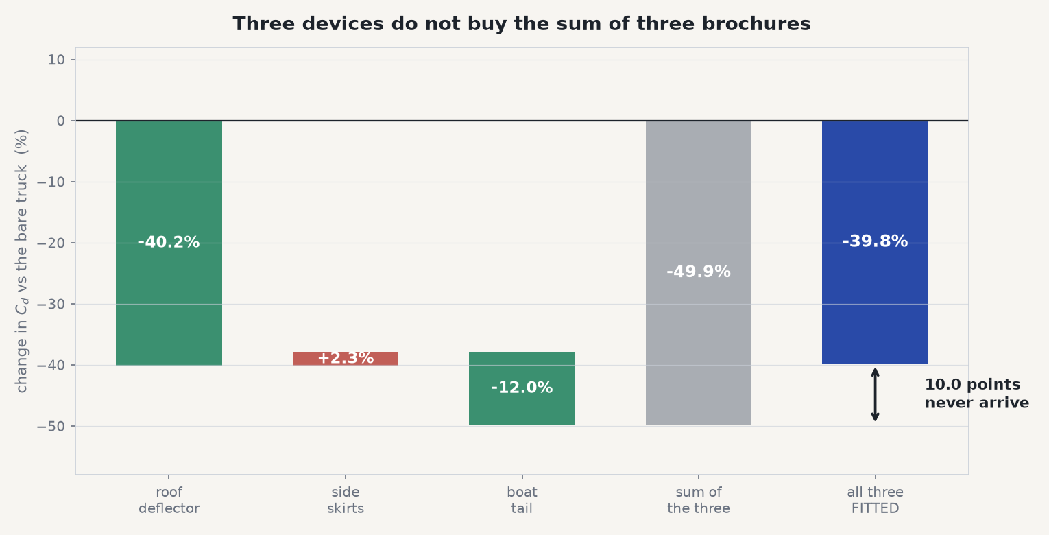
Bar chart: roof deflector minus 40.2 percent, side skirts plus 2.3 percent, boat tail minus 12.0 percent, summing to minus 49.9 percent, against an actual all-three result of minus 39.8 percent. — Each device's individual delta, then the arithmetic sum of the three (**gray**), then the measured all-three case (**blue**). The 10-point gap between the last two bars is not scatter: two devices aimed at the same piece of the flow cannot both remove it.

Take the devices at their individual worth — −40.2 %, +2.3 %, −12.0 % — and the arithmetic promises −49.9 %. Fit all three and the solver returns −39.8 %. Ten points of brochure arithmetic never arrive.

The zone split says where they went. The boat tail's entire benefit was 0.09 of trailer base drag — but with the deflector fitted the trailer's total is already −0.007, so there is no 0.09 left to take. Two devices draw on one account, and whichever is fitted first empties it. Sub-additivity is the result that survives every caveat below, because it describes a relationship between devices rather than any single magnitude.

In fleet money: −49.9 % would be 61.4 kW saved at cruise, and the package saves 49.0 kW. That is 12 kW — some 17 hp — of expected saving that was never there to collect, the difference between a payback model that works and one that quietly does not. The decision it changes is not "is a boat tail worth buying" but "given what is already on this tractor, what does the next device buy?" No datasheet answers that: it depends on the truck, and whichever device goes on first always looks best, because it claims the flow feature they share.

The real-world connection

The strangest number here — a trailer with slightly negative drag — is also the most familiar, because it is the basis of drafting. A cyclist sitting on a wheel saves roughly a third of their power; trucks running close on a highway save both vehicles, the follower most. Same mechanism the deflector exploits: a body that never meets clean, full-pressure air, sitting inside a low-pressure region something ahead of it already paid to create.

The sub-additivity travels further than aerodynamics. Any time two fixes target the same loss they do not add, and the second underdelivers against its own test data — two cooling improvements on one hot component, two noise treatments on one path, two pressure-drop fixes in a duct where a single restriction dominates. Each individual test is honest; the sum is not. And the individual numbers are the ones that exist on paper, so the sum is the one that reaches the business case.

Revisions

v2 · Internal reviewCorrected the y+ statement (24-35 dips below the 30-300 wall-function band), closed the skirts drag split (net +0.018), and added a mesh-resolution limitation; drag results unchanged.

Honest scope. Generic tractor-trailer geometry and three classes of device — no manufacturer's product, no branded geometry, no commercial comparison. Every case is straight-ahead flow at zero yaw, the largest limitation, and it falls hardest on the skirts, whose purpose is a yaw-driven mechanism: the +2.3 % is what a skirt does here, not a verdict on skirts. Stationary ground plane, no wheels and no rotation, so a real part of underbody loss is absent. Half model on the centerline — valid at zero yaw, invalid the moment yaw appears. Steady RANS on a genuinely unsteady wake, each case quoted as a mean with the standard deviation of its per-100-iteration force record: run scatter, not a confidence interval. One mesh per configuration, two of the five re-solved at 2.4× resolution as the refinement check. These counts — roughly 0.3–0.8 million cells on a half model — are well below the tens of millions that production heavy-vehicle CFD uses; the study leans on the edge-fixed separation lines and the refinement check rather than absolute resolution, and the headline is a delta between configurations meshed alike, not an absolute-drag prediction. The tractor improvement is a zone total, so the split between the ramp's own drag and the cab base's recovery is inferred, not measured. Power figures are arithmetic on the modeled C_d (P = ½ρU³C_dA at sea level), not a simulated powertrain, and imply nothing about fuel burn without duty-cycle and efficiency assumptions not made here. Finally, the −40 % is flattered by the baseline: this cab presents a bluff 0.80 m step with nothing filling it, where a modern tractor is better shaped before any retrofit and a fairing added to one is generally credited with nearer 10–15 %. The ranking and the sub-additivity transfer; the headline percentage belongs to this geometry. Three device classes were tested, not the full catalog — no trailer-gap treatment, no mud flaps, no underbody devices.

Fitting a second device, a second cooling fix, or a second stiffener — and you need to know what it is really worth once the first one is already on the machine? The same Ansys workflow behind these five truck solves — one geometry, one recipe, every configuration solved alike, forces resolved per zone so the mechanism shows and not just the total — is how Rand Simulation turns a stack of separate claims into one number you can budget against. That's innovation through insight.