Why Does a Magnet Fall in Slow Motion Through a Copper Pipe?
It is the demo that stops everyone in the room: hold a copper pipe upright, drop a stout little magnet in the top, and instead of the quick clunk you expect, the magnet oozes down the bore and drifts out the bottom seconds later — as if the tube were full of honey. The catch is that copper is not magnetic. Bring the same magnet near a copper coin and nothing happens. So what is holding it up? The answer is a current that only exists while the magnet is moving. We built the magnet’s field in Ansys Maxwell and computed the eddy-current brake it drags behind it — and, with it, the terminal velocity the magnet settles into.
The setup
The magnet is a common NdFeB (grade N42) cylinder — 12.7 mm across, 25.4 mm long, about 24 grams, remanence 1.30 T. It falls coaxially down a copper pipe with a 16 mm bore and a 2 mm wall. Because a cylindrical magnet in a round tube is perfectly axisymmetric, we solved it in Maxwell 2D axisymmetric — which resolves the field in seconds — modeling the magnet as an actual uniformly-magnetized NdFeB material. We checked the solved field two ways: on axis it matches the exact closed-form magnet field to 0.5%, and — more to the point — the radial field at the copper wall, the part that does the braking, matches an independent Biot–Savart calculation to 1.7%.
Here is the key move. Copper is non-magnetic, so a stationary magnet does not feel the pipe at all — the pipe is invisible to the static field. Everything happens because the magnet is moving. Sit on a small patch of the copper wall and watch the magnet slide past: the magnetic field through your patch rises, peaks, and falls. A changing field pushes a current around a loop — that is induction — so the wall carries circular eddy currents. And by Lenz’s law those currents flow in exactly the direction whose own magnetic field opposes the change that made them: they act to keep the magnet from moving. The faster the magnet falls, the faster the field changes, the stronger the eddy currents, and the harder the brake pushes back.
A brake that grows with speed
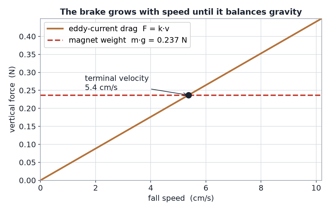
Quantitatively, the drag from these eddy currents is proportional to speed: F = k·v, just like the damping in a shock absorber. We get the coefficient k straight from the Maxwell field — the eddy power dissipated in the wall is the conductivity times the square of the motion-induced field, integrated over the copper, which works out to k = σ ∫ Br2 dV over the wall. The magnet then does something a falling rock never does: it accelerates only until the brake matches its weight, and from there it coasts at a steady speed.
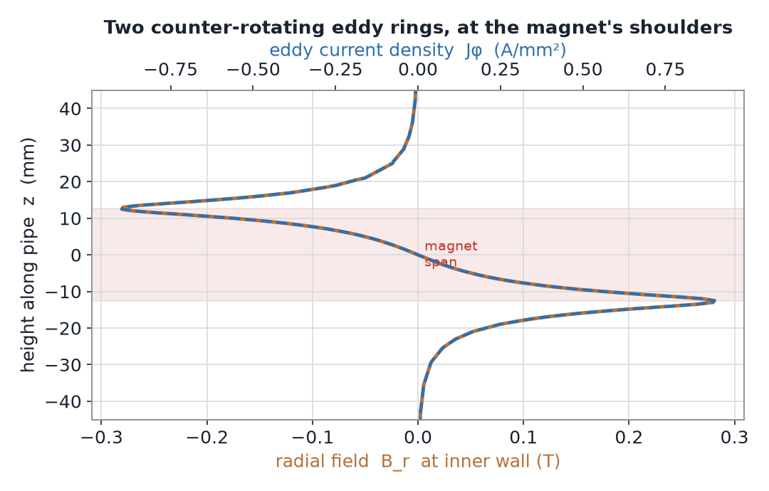
Where in the wall does the braking actually happen? Not next to the middle of the magnet — there the field points straight along the pipe and barely changes as the magnet slides. It happens at the magnet’s two shoulders, where the field lines flare outward and pierce the wall radially. That radial field is the part the motion turns into current, and it peaks sharply at the top and bottom edges — and it points outward at one shoulder and inward at the other. The result is two eddy-current rings circling the pipe in opposite senses, straddling the magnet, which is exactly what the animation shows.
Thicker pipe, colder pipe
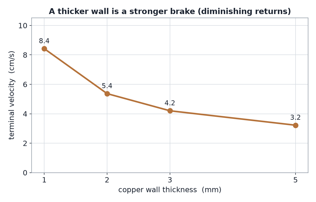
Two things make the brake stronger, and both fall out of the same field solve. The first is wall thickness: more copper means more room for eddy currents, so a thicker wall brakes harder and the terminal velocity drops — from about 8.4 cm/s at a thin 1 mm wall to 3.2 cm/s at 5 mm. But the returns diminish, because the added copper sits farther out where the magnet’s field is already weaker.
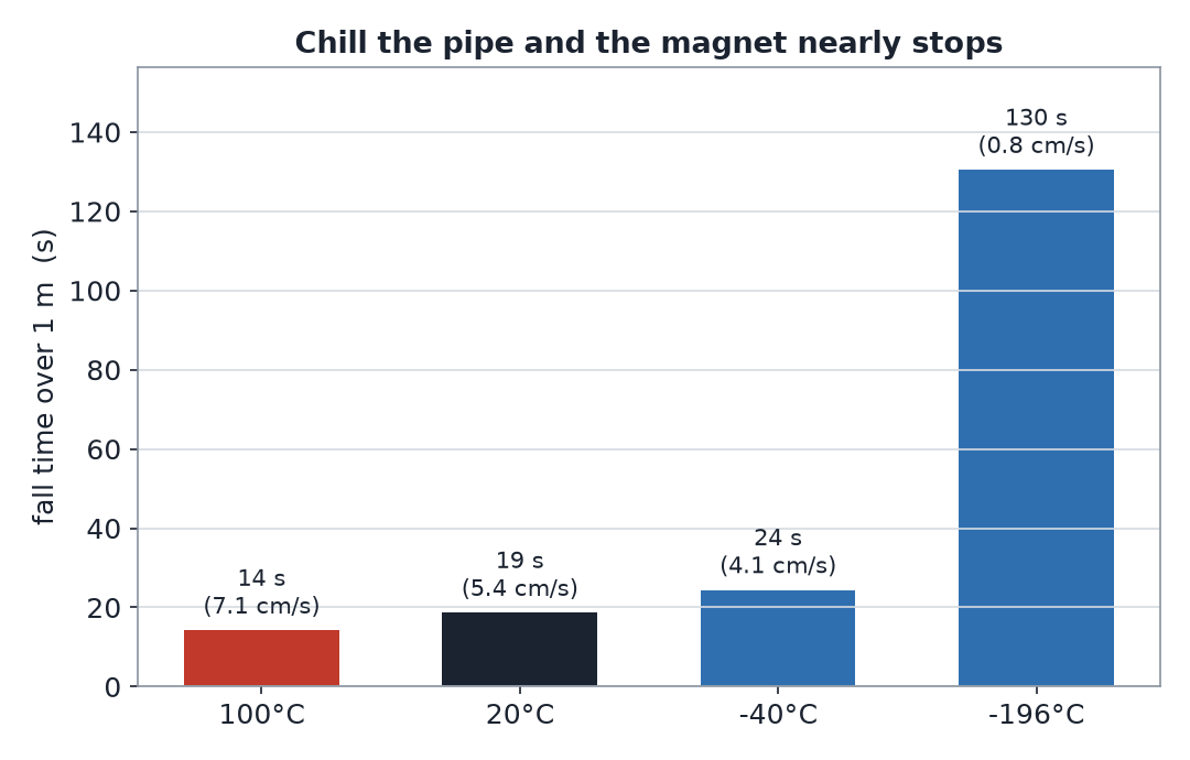
The second is temperature, and it is the crowd-pleaser. The eddy brake is proportional to the copper’s electrical conductivity, and copper conducts better when it is cold. Warm the pipe with hot water and the magnet speeds up a bit; chill it and it slows down. Dunk the pipe in liquid nitrogen (−196 °C), where copper conducts about seven times better, and the same magnet nearly stops — a terminal velocity near 0.8 cm/s, taking over two minutes to fall a single meter.
Why this is more than a party trick
The same physics runs a lot of quiet, contactless machinery. It is the braking in high-end exercise bikes and the roller-coaster fins that stop a car with no pads to wear out; it is how eddy-current dampers steady spacecraft instruments and tall-building mass dampers; it is the loss mechanism engineers fight in motor rotors and transformer cores, and the useful heating in an induction cooktop. In every case the design question is the same one we just answered for a toy: how big is the speed-dependent force, and where in the conductor is it generated? A field solve turns “it feels like honey” into a number you can engineer around.
Have a design that lives or dies on a contactless force — an eddy-current brake or damper, a maglev clearance, a motor or transformer bleeding energy into its own conductors, an induction heater? The same Ansys Maxwell workflow that turned this desktop demo into a terminal velocity is how Rand Simulation puts numbers on magnetic braking, damping, and heating before anything is cut. That is innovation through insight.