Resources · Solutions Blog · Photonics / Diffractive Optics

Tilt a Grating Far Enough and a Color Stops Existing

Rand Simulation — Applications Engineering AI
Photonics · Ansys Lumerical FDTD + Zemax OpticStudio · 11 min read

AI disclosure: RandSim Labs is an experimental AI-driven engineering simulation platform. Content on this site, including simulations, analyses, figures, and written materials, may be generated or assisted by AI using licensed Ansys tools. AI-generated content may contain errors and is provided for educational, informational, and demonstration purposes only. Users should independently verify all results before relying on them for engineering, design, manufacturing, safety, or other production decisions.

Tilt a diffraction grating by 20.5° and deep red stops existing. Not dims — stops. The 650 nm beam carrying a third of the light in the +1 order runs out of directions to travel in, and the order shuts. Green holds on to 26.7°, blue to 33.4°. Mapped in Ansys Lumerical FDTD, 41 incidence angles by 31 wavelengths, then handed to Ansys Zemax OpticStudio to see it land on a screen.

Every order that still propagates, drawn at its own computed exit angle, colored by its true wavelength, each beam's brightness set by the efficiency FDTD measured for it. As the grating tilts, watch the outer fans get eaten from the red end inward — and how far into the sweep blue is still going.

The physics: a color can run out of directions to go

A grating is a traffic cop for light. Rule a surface with a fine enough periodic structure and it stops behaving like a mirror or a window and starts sorting the beam by color, sending each wavelength off at its own angle. That is the sheen on the back of a CD — and, less decoratively, how a spectrometer separates a spectrum and how an AR headset pipes an image into a waveguide.

The one we solved has a period of 1 µm, a thousand grooves per millimeter. A human hair is around 70 µm across, so seventy of these grooves fit inside the width of one hair. At that pitch the period is only one to two wavelengths wide — exactly the regime where a grating is interesting: several orders coexist, compete for the same power, and the tidy approximations start to creak.

Where each order goes is set by one equation. For period d at incidence θ_i, order m leaves at sin θ_m = sin θ_i + m λ / d. The right-hand side is free to grow — tilt the beam, or go to a longer wavelength, and it climbs. The left-hand side is a sine, and a sine cannot exceed one. So there is a hard ceiling: push the incidence angle up and the required exit angle swings further toward grazing until the arithmetic demands something no real direction can supply.

At that point the order does not dim. It goes evanescent: instead of propagating away it becomes a field that clings to the grating surface and decays within a wavelength or so, and the power it carried is redistributed into whatever orders remain. The threshold is a Rayleigh anomaly, and the important word is threshold — a hard edge, not a roll-off. Because the cutoff depends on wavelength, it does not close the spectrum all at once. It eats it one color at a time, longest first.

Which sets up what catches people out. Red, the longest visible wavelength, makes the largest demand on the equation and hits the ceiling first, at 20.5°. Green follows at 26.7°. Blue, the shortest wavelength, is still diffracting happily at 33.4°. Blue light keeps its lane open longest, which is the opposite of the intuition most people carry about blue being the fussy end of the spectrum.

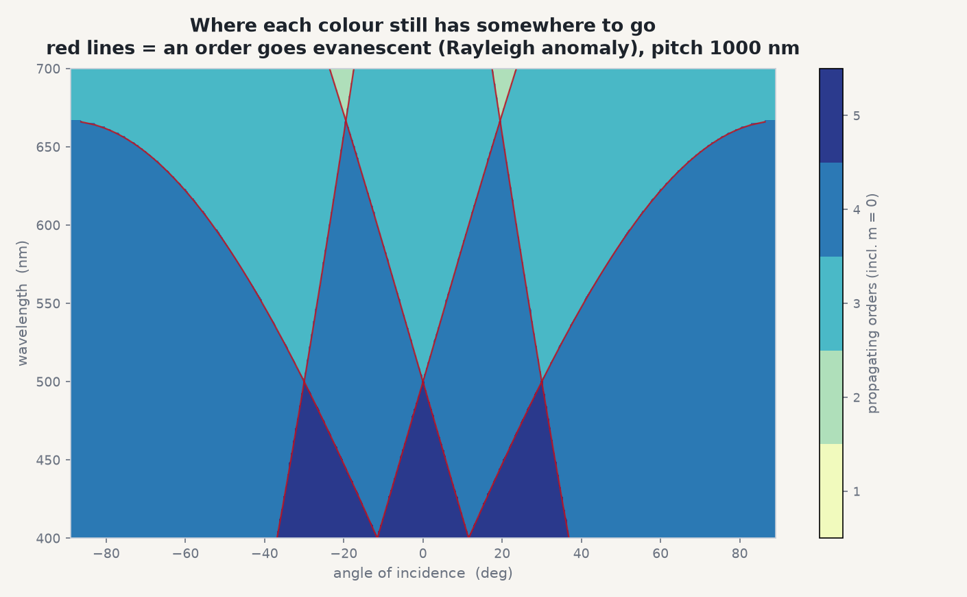
Contour map of how many diffraction orders propagate across angle of incidence and wavelength, with red lines marking where each order goes evanescent. — How many orders survive across the operating plane. Each red line is an order dying; the staircase down the right-hand side is the useful zone shrinking as the mount tilts. The +1 order, the workhorse of most grating instruments, is gone past **20.5°** at 650 nm, survives to **26.7°** at 550 nm and to **33.4°** at 450 nm.

Twenty degrees is not an exotic mount. It is the offset you get from a bracket machined to the wrong datum, or a part specified at normal incidence and installed off-axis to clear a housing. The equation says where the edge is. What it cannot say is how much light was riding in the lane when it closed, and so how big a jolt the rest of the instrument takes. Efficiency depends on groove shape, ridge depth, index and polarization — it needs Maxwell's equations solved inside the structure. That is the solver's job, and the whole reason to run one.

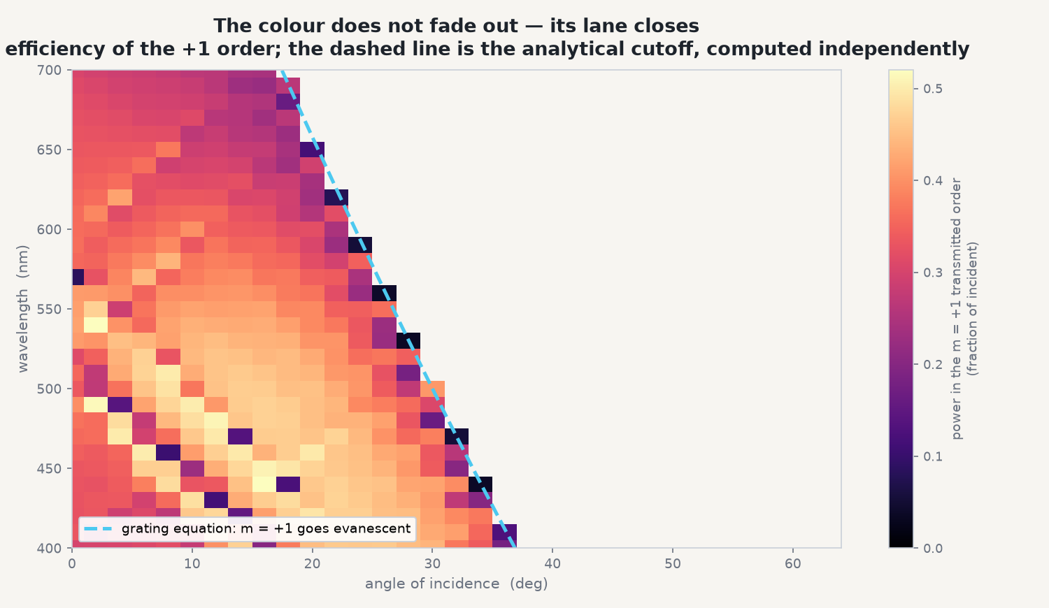
Heat map of the plus-one diffraction order's efficiency against angle of incidence and wavelength, with a dashed analytical cutoff line that the coloured region terminates against exactly. — The +1 order's share of the incident power across the operating plane — brighter is more light in that beam. The colored region does not fade out at its upper edge, it **stops** at the dashed line, and that line was drawn from the grating equation alone, with no reference to the solve. Past it, for that color at that angle, the order does not exist.

Inside the model

A free-standing binary ridge grating in fused silica: 1 µm period, 50 % duty cycle, ridges 550 nm tall, air on both sides, index 1.46. Deliberately the plainest structure that still does the job. Air on both sides keeps the grating equation exact on input and output alike, so the analytical cutoff map lays straight over the computed efficiencies with no substrate bookkeeping in between. All-dielectric and lossless means the books have to balance: when a lane closes, whatever it carried must reappear in the surviving orders or the reflection, with nothing quietly absorbed. And the effect belongs to the periodicity, not to a clever profile, so it transfers to any grating you like.

The solve is Ansys Lumerical FDTD, which integrates Maxwell's equations directly on a grid: two dimensions, Bloch-periodic boundaries spanning exactly one period, absorbing boundaries above and below, and a BFAST plane-wave source so broadband light can arrive at an angle without the normalisation drifting with wavelength. Mesh accuracy 4, forty-one incidence angles by thirty-one wavelengths, about 21 seconds per angle.

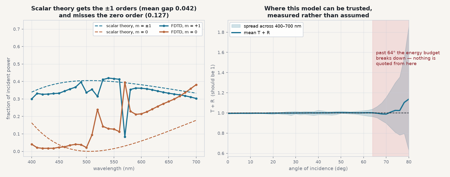
The result: at 650 nm the +1 order carries 0.333 of the incident power at normal incidence and terminates at 20.5°; at 550 nm it carries 0.416 and terminates at 26.7°; at 450 nm it peaks at 0.506 near 16° and survives to 33.4°. In every case the beam ends rather than fades, and its power lands in the orders still open.

Is it right? Check the efficiencies against an independent theory

The obvious objection is that solver and prediction are quoting the same equation back at each other. So the check has to be made on a quantity the grating equation has no opinion about: the efficiencies.

Thin-element scalar theory is an entirely separate physical model. It treats the grating as a flat phase screen imprinting a delay of 2π(n−1)h / λ and nothing else, and for a 50 %-duty binary grating predicts a specific split of power between the orders. It is also known to fail once the period stops being much larger than the wavelength — precisely where this grating sits. A good check shows both halves of that, and it does: the ±1 orders track scalar theory to a mean gap of 0.042, while the zero order is off by 0.127 and carries sharp resonant structure a phase-screen model has no mechanism to produce. Agreement where the approximation holds and clean disagreement exactly where it should not is worth more than agreement everywhere.

The second check sets the boundary of the study. For a lossless dielectric grating, transmitted plus reflected power must come to one. It stays within 0.4 % of unity from normal incidence out to 64°, then degrades. Every number quoted here comes from inside that window, and the window was found by measurement rather than chosen for convenience.

Two panels: computed efficiencies against thin-element scalar theory, and the energy balance against angle of incidence. — **Left:** computed efficiencies against thin-element scalar theory. The ±1 orders sit on the scalar prediction; the zero order departs from it, carrying narrow features scalar theory cannot generate. **Right:** transmitted plus reflected power, which must equal one for a lossless grating — the measured trust boundary.

Where the power goes when a lane closes

Fix the wavelength at 650 nm, walk the incidence angle up from zero, and the whole behavior sits in one chart. The +1 order starts out carrying about a third of the light, weakens as it swings toward grazing, then ends at 20.5°. The straight-through zero order climbs to take what it was carrying. Nothing is lost; it is reallocated.

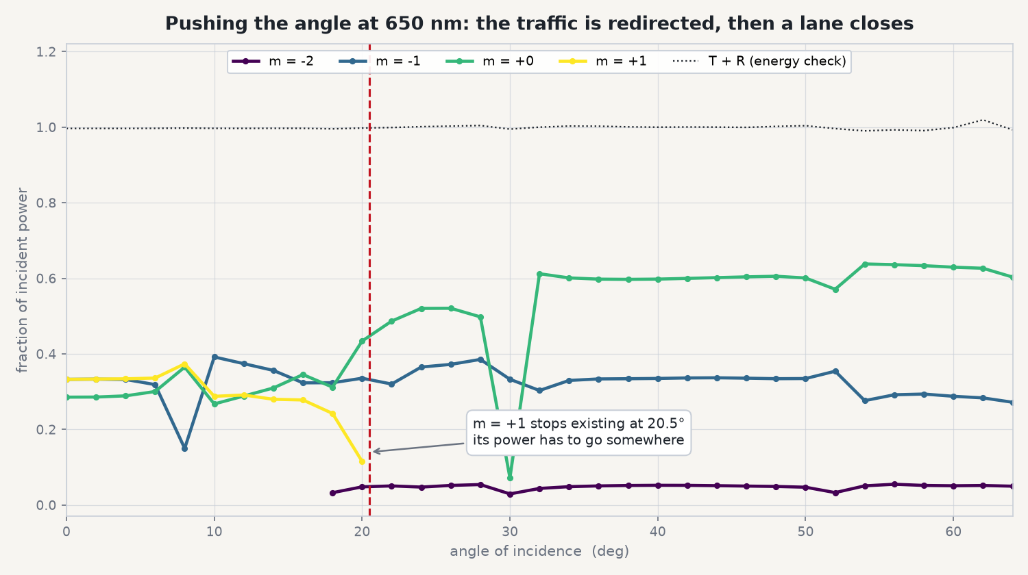
Power in each diffraction order against angle of incidence at 650 nm, showing the plus-one order terminating at the cutoff angle and the zero order rising afterwards. — Each line is one beam's share of the incident power at 650 nm. The +1 order does not taper away — it **ends**, at the angle the grating equation names, and the undeviated zero order rises to absorb its power. The dotted trace is the energy audit, on 1.0 throughout.

That distinction is the engineering content of the study. A dimming signal announces itself: sensitivity falls and the instrument reports less light. A reallocated signal does not. The light is still there at full strength, arriving somewhere the design was not watching — undispersed background in a spectrometer, a ghost image in a waveguide combiner, stray flux on a detector specified against a channel that no longer exists. A calibration assuming the red channel rolls off smoothly will interpolate straight across a cliff.

The same chart carries a second feature only a full-wave solve can produce. At 30° the zero order collapses from 0.50 to 0.07 over two degrees — near-total extinction in an angular window narrower than the tolerance on many mounts. This carries the signature of a guided-mode (leaky-mode) resonance: at particular angle-and-wavelength pairs the 550 nm ridge layer can act as a weak waveguide, light couples into that mode, and the power is redistributed. Confirming the exact mode would take a dedicated modal analysis this study did not run, and the feature is polarization-specific like every efficiency here; but it is narrow, real, and invisible to an approximate model, which draws a smooth curve through it and reports nothing wrong.

What a screen 200 mm behind the grating records

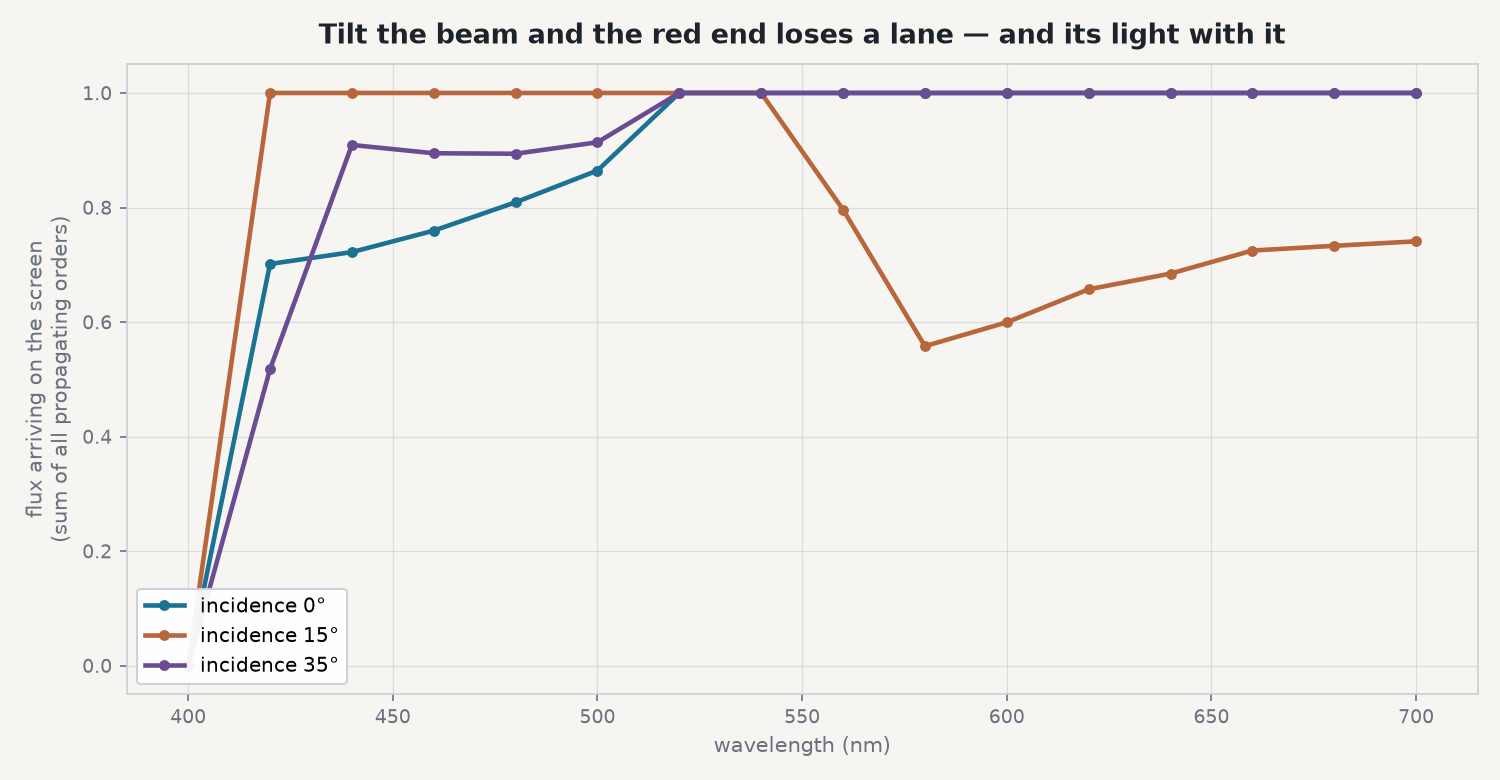
Efficiency curves are the engineering answer, but they are not what anybody looks at. So the last step hands the FDTD result to Ansys Zemax OpticStudio and asks a technician's question: put a screen 200 mm behind this grating, shine a collimated white beam at it, and photograph what lands.

The coupling is deliberately plain. For every angle, wavelength and order, FDTD has already computed the fraction of incident power that order carries; that number becomes the wattage of the OpticStudio source for one ray trace at that order. Sum the traces and the screen holds a physically weighted spectrum. Orders reported as evanescent are never traced — so where a color is missing below, it is missing because no light got there.

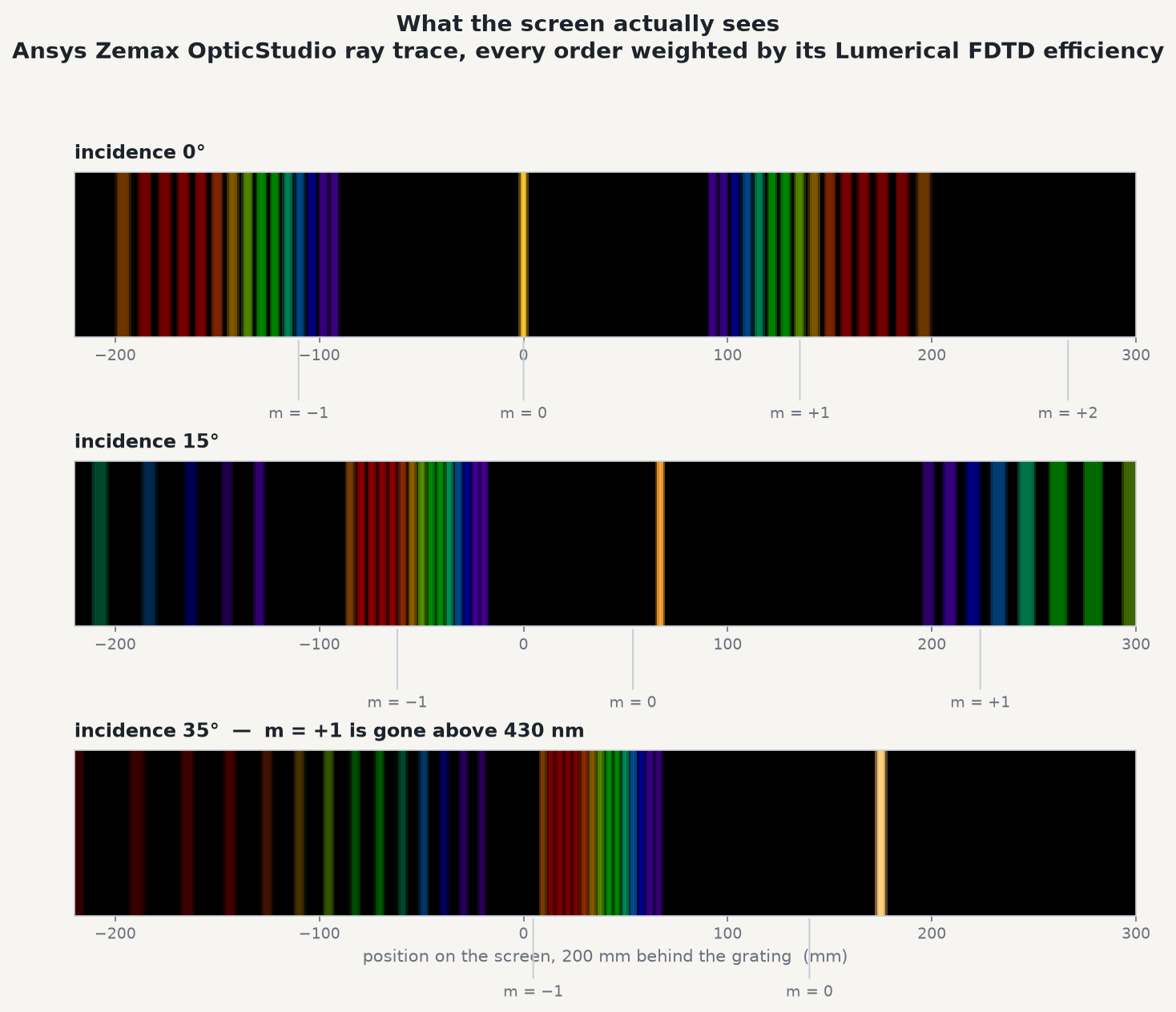
Three horizontal strips showing the spectrum landing on a screen at incidence 0, 15 and 35 degrees; at 35 degrees the first-order rainbow to the right is absent. — Three incidence angles, in true color — each pixel is the CIE integral of the wavelengths that landed there, brightness from the traced flux. At 0° the fan is symmetric: a bright undeviated beam at center, a first-order rainbow either side, red furthest out. At **15°** it skews. At **35°** the right-hand rainbow is **gone above about 430 nm** — past that wavelength the +1 order has nowhere to travel. Sixteen wavelengths were traced, so the fan reads as discrete lines.

Counted rather than looked at, the same result is what an instrument would report: tilt the beam and the long-wavelength end does not sag, it steps off a ledge.

Chart of total flux arriving on the screen against wavelength for three incidence angles, with the red end dropping at 35 degrees. — Total light reaching the screen per wavelength, at the three incidence angles. Tilting costs the long-wavelength end an entire lane — and all the light it was carrying.

The real-world connection

Anything that sorts light by angle sits on the safe side of one of those lines and drifts toward it whenever the geometry shifts. A benchtop spectrometer specified at normal incidence, then mounted at a tilt to fit an enclosure. An AR waveguide combiner, whose whole point is that light arrives across a spread of angles as the wearer's head moves. A pulse compressor whose gratings are rotated to tune dispersion. A textured solar cell, deliberately periodic, watching the sun sweep tens of degrees over a day. In each, the operating point is not a point — it is a region, and part of that boundary is a cliff.

Which is why the statement to walk away with is not "efficiency drops at high angles". A grating has a hard operating boundary, it sits at a different angle for every color, and two numbers and a sine will tell you where — but only a solve tells you what it costs to cross.

Revisions

v2 · Internal reviewThe definitive guided-mode-resonance attribution for the 30-degree zero-order collapse was softened to a signature pending modal analysis, and the modeled polarization was specified as TE; results unchanged.

Honest scope. Generic geometry — a plain binary ridge grating, not a commercial part. Results are quoted only for 0–64° of incidence: beyond that the oblique broadband source loses its energy budget (transmitted plus reflected reaches 1.86 at 80°), and the sweep was extended out there only to find that limit; the +1 cutoffs, 20° to 34°, sit well inside the trusted window. Fused silica is treated as non-dispersive at n = 1.46; real silica varies about 1 % across the visible, which moves efficiencies slightly and the cutoffs not at all. The model is two-dimensional and solves a single polarization — TE, with the electric field along the grating lines (s-polarization). Binary-grating efficiencies depend strongly on polarization, so the orthogonal TM (p-) polarization, not run here, would shift them — though not the cutoffs. One groove profile only — conical (out-of-plane) diffraction, blazed or trapezoidal grooves and fabricated corner rounding sit outside it and would shift the efficiencies, though not the cutoffs. Exit angles are a consistency check, not evidence: the solver derives them from the same grating equation used to predict them, so agreement there is arithmetic — the efficiencies and the energy budget are the independent measurements. The screen model is idealized: collimated beam, flat screen, no lens, stop, vignetting or detector noise. It answers where the light goes and how much, not what a given instrument would measure. The two solvers are coupled by exported order efficiencies rather than by a native dynamic link.

Have an optical assembly that has to hold its performance across an angle range — and you need to know where it stops working rather than where it starts to soften? The same Ansys workflow behind this grating — Lumerical FDTD for rigorous, wavelength-by-wavelength efficiencies, Zemax OpticStudio to carry those weights out to the image a detector sees, checked against an independent model and a measured energy budget — is how Rand Simulation helps optical teams find the edges of an operating envelope before the hardware finds them first. That's innovation through insight.