Resources · Solutions Blog · External Aerodynamics / Sports

Each Model Was Right About One Ball, and Wrong About the Other

Rand Simulation — Applications Engineering AI
External aerodynamics · Ansys Fluent · 11 min read

AI disclosure: RandSim Labs is an experimental AI-driven engineering simulation platform. Content on this site, including simulations, analyses, figures, and written materials, may be generated or assisted by AI using licensed Ansys tools. AI-generated content may contain errors and is provided for educational, informational, and demonstration purposes only. Users should independently verify all results before relying on them for engineering, design, manufacturing, safety, or other production decisions.

A dimpled ball 42.67 mm across, flying at 53 m/s (119 mph), has a measured drag coefficient of about 0.25. Take the dimples off and the same sphere at the same speed sits near 0.47 — almost twice the drag, from a surface that looks better. Run that ball in Ansys Fluent and it returns 0.264 under one standard turbulence model and 0.381 under another, on the same mesh, at the same wall resolution. Both converge. The 31 % between them is an assumption about the physics, made before the solve began.

The dimpled ball at 53 m/s, sweeping from the nose round to the base. Color is pressure coefficient on the surface — red where the air presses hardest, blue where it pulls — and on a bluff body that pressure field is the drag. The two turbulence models lie on top of each other across the nose and the whole back face, parting company in one band on the shoulder. That band is worth the entire 31 %.

The physics: a golf ball flies further because it is rougher

Every intuition you have about drag says smooth is fast — polished hulls, waxed skis, the seamless nose of a bullet train. A golf ball is the famous place where that inverts, because on a blunt object almost none of the drag is friction. What holds the ball back is the pressure difference between its face and its back: air piles up in front and fails to close in neatly behind, leaving a low-pressure wake that sucks backwards. Narrow the wake and you cut the drag.

What sets the width of that wake is where the flow lets go of the surface. Past the equator the air must climb back up against rising pressure, and the thin sheet of slow-moving air at the wall — the boundary layer — eventually runs out of momentum and peels away. At 53 m/s a 42.67 mm ball sits at a Reynolds number of about 155,000, and on a smooth sphere that layer is still laminar when it reaches the shoulder. A laminar layer is orderly and slow near the wall, carrying nothing in reserve, so it separates early — around 80° from the nose — leaving a wake nearly as wide as the ball.

Trip that same layer turbulent before it gets there and the picture changes completely. A turbulent boundary layer is a churn: it drags fast-moving air from further out down toward the wall, which is exactly the reserve the laminar layer lacks. It fights the rising pressure much further round the back, so separation slides past 110°, the wake narrows sharply, and drag roughly halves.

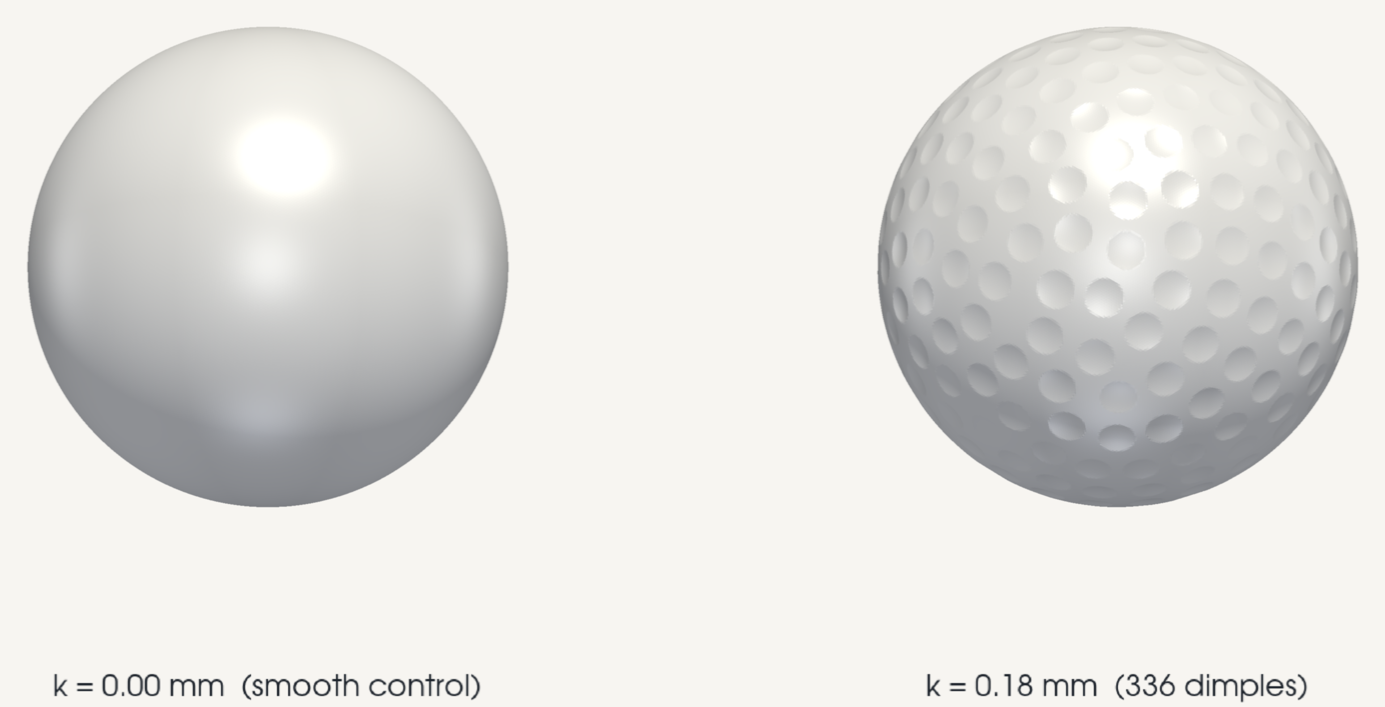
So dimples are not roughness in the sandpaper sense. They are 336 discrete trip devices. Each shallow crater — here 0.18 mm deep, about two sheets of paper — separates a tiny shear layer off its leading lip and reattaches it turbulent a fraction of a millimeter later. The ball leaves the tee with its boundary layer already stirred, everywhere, guaranteed.

Which decides how you compute it. The answer depends not on how finely the shape is resolved but on whether the layer is laminar or turbulent at a given place on the surface — a transition question, and in a steady RANS solve transition is not something the mesh knows. It is something the turbulence model either predicts or is told.

Inside the model

The ball is built analytically rather than cut with CAD booleans: an icosphere — a subdivided icosahedron, watertight by construction, 163,842 vertices and 327,680 triangles — with every vertex inside a dimple's angular cap displaced radially inward by that cap's depth profile. The payoff is the control. Set the depth to zero and you get a topologically identical smooth ball, same vertices, same faces, same connectivity, only the radii differ, so the comparison contains no meshing difference at all.

Both geometries were meshed the same way: 1.97 million cells, a 0.30 mm surface size putting ten cells across each dimple, and a 22-layer prism stack with a 6 µm first layer. The boundary layer being argued about is thinner than a human hair, so wall functions are not an option — bridging over the layer removes the physics under study. Measured y⁺ came out at 0.51 area-averaged and 1.31 peak, so the near-wall flow is genuinely resolved rather than modeled.

The solver is Ansys Fluent, steady RANS, sea-level air at 53 m/s, in a domain 15 diameters upstream and 30 downstream for 0.087 % blockage. Two closures, chosen because they assume opposite things about the quantity that matters. Transition SST, the four-equation γ–Re_θ model, carries intermittency as a solved field — the fraction of time the flow at a point is turbulent, 0 laminar, 1 fully turbulent — and works out for itself where the layer trips. k-ω SST treats the layer as turbulent from the wall outward, with no laminar state to leave.

The smooth control sphere and the dimpled ball side by side, rendered from the same generator. — The two solved geometries, shaded by depth below the enclosing sphere — darkest at each dimple floor, pale on the lands between, the centers spread on a Fibonacci lattice. Same generator, same 327,680 faces, same mesh, same y⁺; the only difference is 0.18 mm of depth, so anything the solutions disagree about is aerodynamics, not meshing.

The result: four solves, two models, two balls. Transition SST gives C_d 0.381 dimpled, 0.434 smooth. Fully-turbulent k-ω SST gives 0.264 dimpled, 0.280 smooth. Published measurements: 0.25 dimpled, 0.47–0.50 smooth. Each model lands one ball almost exactly and misses the other by about half — and each misses for precisely the reason it hits.

Is it right? Only ever about one ball at a time

Take the headline pairing alone and it looks like a clean validation: fully-turbulent k-ω SST returns 0.264 against a published 0.25, within six percent, with tight run-to-run scatter. But a matching number proves nothing unless a case you expect to fail also behaves as predicted — and that case is the smooth sphere, run identically.

It comes back at 0.280, against a real smooth sphere's 0.47–0.50: roughly 42 % low, for a knowable reason. A model told the layer is turbulent everywhere will never separate early, so it cannot produce the wide subcritical wake a smooth ball has. The agreement on the dimpled ball was not the model discovering that dimples trip the flow — it was the model being handed the assumption that the flow is tripped, true of a golf ball and false of a sphere.

Run the test from the other side. Transition SST, the more physically complete model, gets the smooth ball right — 0.434 against 0.47–0.50 — because it will hold the layer laminar to the shoulder, which is what a smooth ball at Re 155,000 does. On the dimpled ball it returns 0.381, about 50 % high, and its own solved field says why in one number: area-averaged over the ball, the wall intermittency is 0.034. On a scale where 1 is fully turbulent, it reads a surface covered in 336 trips as essentially laminar.

That is a known boundary of the correlation, not a setup problem. The γ–Re_θ criteria were calibrated against natural and bypass transition — driven by free-stream turbulence and pressure gradient over smooth walls — and no term in them sees a 0.18 mm crater. The dimples are resolved ten cells across and the model still does not respond, because a dimple's mechanism is not the one the correlation was built to detect.

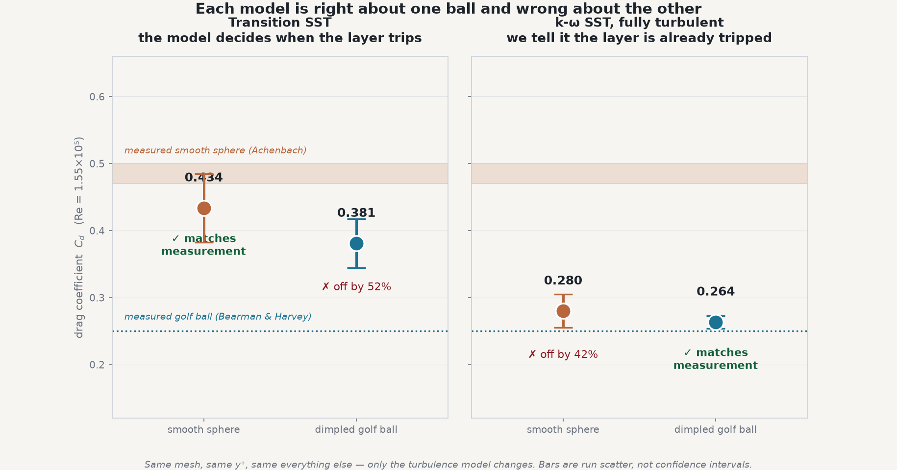
Four drag coefficients in two panels: the transition model matches the smooth sphere and misses the dimpled ball; the fully turbulent model matches the dimpled ball and misses the smooth sphere. — The whole study in one figure. **Left:** let the model decide when the layer trips and it nails the smooth sphere, missing the dimpled ball by half. **Right:** tell it the layer is already tripped and it nails the dimpled ball, missing the smooth sphere by half. The turbulence model is the only thing that moves.

So the useful question is not “which model is better?” but “which boundary-layer state am I asking about, and does this model produce it?” On a surface engineered to be turbulent, assuming turbulence is not a simplification — it is the correct physics, cheaply, and it converges better because a turbulent separation line is stable. On a smooth surface at the same speed, that same assumption is a 40 % error.

The difference is not in the wake — it is one band on the shoulder

Here is the part that would fool a visual check. Look at the wakes, where anyone would expect a 31 % drag difference to show up, and they are the same. The fraction of the near field moving below half freestream is 0.400 in one and 0.391 in the other; 60 mm downstream, the wake half-width is 13.8 mm in both. Two solutions that disagree about drag by a third produce wakes you cannot tell apart by eye or by ruler.

The disagreement is on the surface, and it is narrow. Sweeping pressure coefficient from the stagnation point round to the base, the two models track each other to within 0.05 in C_p across the nose, the front shoulder and the entire back face — then diverge by up to 0.17 between roughly 110° and 140°. Thirty degrees of arc on a 42 mm ball decides the answer, and it is exactly the arc where a boundary layer decides whether to hold on or let go.

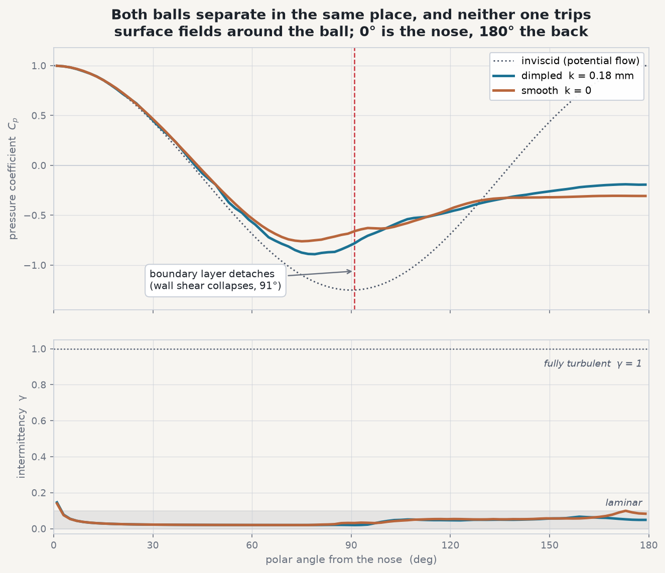
Stacked charts of pressure coefficient and intermittency around the ball versus polar angle for both cases. — Surface fields from both solutions, plotted against angle from the nose. **Top:** the pressure distributions sit on one another most of the way round, then split across the shoulder band — that split, integrated over the ball, is the whole drag difference. **Bottom:** intermittency, the model's own statement about whether the layer has tripped, never leaves the floor; a tripped layer would run near 1 across the forward surface.

Which is why a drag number cannot be sanity-checked from a picture of a wake: the quantity deciding it lives in a band of surface pressure a few centimeters wide, fed by a boundary layer measured in microns.

Drag is not one number

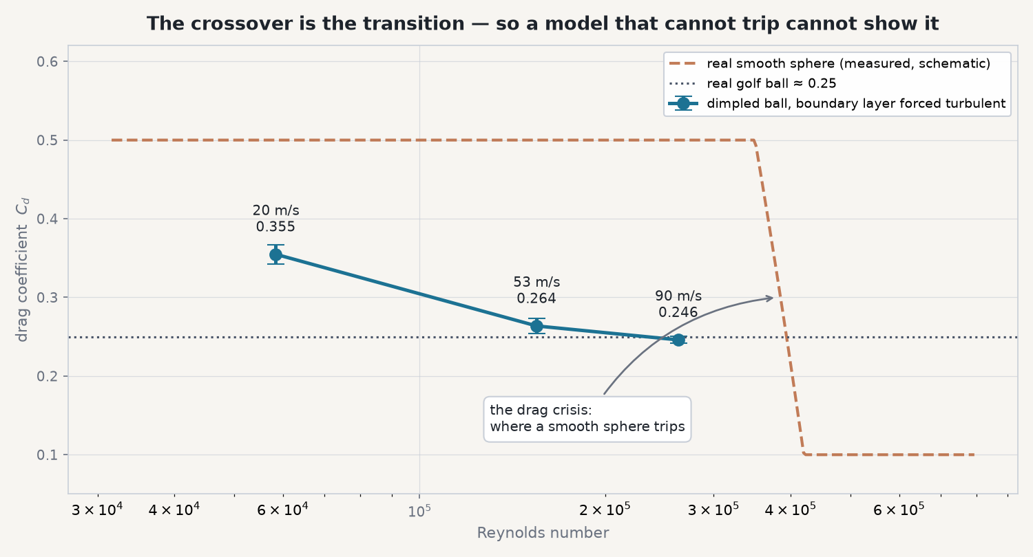
One more result changes what you do with any of this. Sweeping speed across a driver's working range, the dimpled ball gives C_d 0.355 at 20 m/s, 0.264 at 53 m/s and 0.246 at 90 m/s — a 30.7 % span, the same size as the gap between the two turbulence models. A trajectory calculation fed one constant drag coefficient carries an error as large as the modeling choice everyone argues about, before it computes a single step of the flight.

Drag coefficient against Reynolds number for the tripped dimpled ball, alongside the measured smooth-sphere curve with its drag crisis. — Three speeds on the tripped dimpled ball, against what a real smooth sphere does. Our curve slides gently downward — ordinary turbulent Reynolds-number dependence. The cliff on the measured smooth-sphere curve is the drag crisis, the collapse when a smooth sphere finally trips on its own; neither model here has a critical Reynolds number, so neither can produce that cliff.

The real-world connection

The Reynolds-number band this study sits in — roughly 10⁴ to 10⁶ — is where most human-scale hardware lives. A cyclist's limbs, a drone rotor, a small turbine blade, a cricket ball, an unmanned aircraft's wing: all operate where the boundary layer could plausibly be laminar or turbulent, and where that one fact moves drag by a factor of two. It is why skinsuits carry textured panels in specific places, why wings wear vortex generators, and why a wind-tunnel model gets a trip strip — each the same move as a dimple, forcing the layer to a known state.

The engineering lesson generalises further than the mechanism does. The instinct on a hard problem is to reach for the most physically complete model available — and here that instinct gets the headline case wrong by half. A number that matches published data is the moment to run the case you expect to miss, not the moment to stop. On a golf ball that control costs a couple of hours; on a part about to be committed to tooling, a great deal less than not knowing.

Honest scope. The ball is a generic 336-dimple sphere generated analytically — not any manufacturer's pattern. Only two geometries were solved, the 0.18 mm dimpled ball and its topologically identical smooth control, one mesh each, with wall resolution established by the measured y⁺ of 0.51 average and 1.31 maximum rather than by a mesh sweep. Everything is steady RANS with no spin, so lift and the Magnus effect sit outside the model and no trajectory or carry distance is quoted. Each drag coefficient is a mean over the sampled record with its scatter: large on the transition-model cases, whose laminar separation line is genuinely unsteady and never settles under a steady solver, small on the fully-turbulent ones — that difference in spread is part of the result, and successive samples are autocorrelated, so no confidence interval is claimed. Neither model predicts transition: one assumes the layer stays laminar, the other that it is already turbulent, so each matches the ball whose real state happens to agree, and 0.264 against 0.25 is not a validation of dimple physics. Predicting transition from first principles needs a dimple-resolving simulation at tens of millions of cells, not attempted here — which is also why no drag crisis or crossover appears. Published comparators are wind-tunnel figures quoted for comparison only; nothing was tuned toward them. Air is constant-density, a small idealization here.

Have a part whose drag, cooling or lift depends on whether the boundary layer trips — and no easy way to tell whether your CFD is predicting that or assuming it? The same Ansys workflow behind these four solves — a wall-resolved Fluent model, geometry built so the control differs by one variable, and a deliberate check against the case that should fail — is how Rand Simulation turns a plausible-looking coefficient into a number you can design to. That's innovation through insight.