A Chicago Drive-Time Map, Solved as Heat Conduction
Everyone has stared at a map and wondered how far they could get in half an hour. Here is an odd way to answer it: mesh a real city’s streets, make every road conduct heat in proportion to its speed limit, warm up downtown, and watch the heat pour outward. The glow that spreads along the grid is the drive-time map — freeways run hot and race ahead, side streets amber in slowly behind. We built it in Ansys, and then spent most of our effort on the honest part: turning that glow into minutes a driver would actually recognize.
Why heat, of all things
A street network is a graph: intersections joined by road segments, each with a length and a speed limit. That is exactly the shape of a one-dimensional heat-conduction problem — a lattice of little conducting bars meeting at shared nodes. Ansys Mechanical’s thermal solver assembles the network’s conduction matrix and marches it forward in time; nothing hand-computes the physics, the solver does. So the question “where does the warmth reach by time t?” becomes a stand-in for “where can you drive by time t?” — if we wire the analogy up correctly.
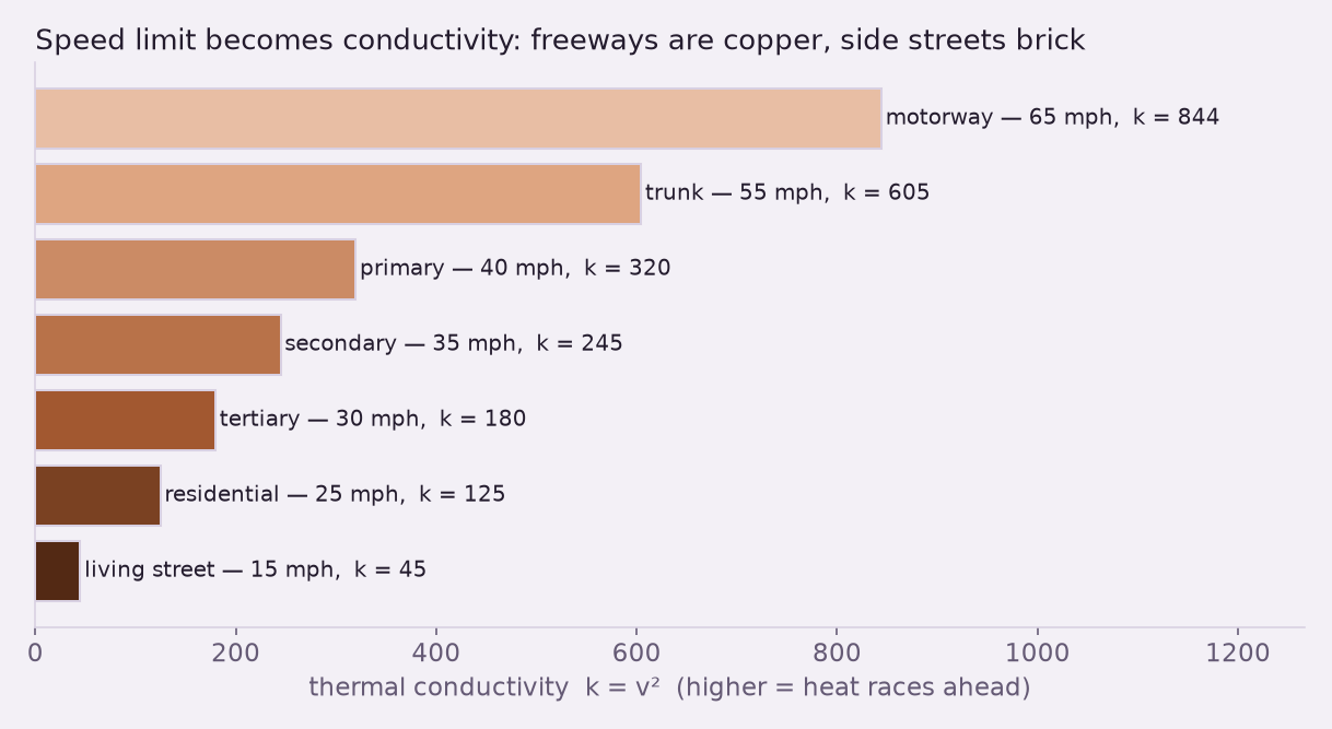
The wiring is one idea. Heat spreads fast where a material conducts well, so a road’s conductivity has to encode its speed. Give every segment a conductivity equal to the square of its speed limit, keep the heat capacity uniform, and the diffusion “distance” along the network becomes the travel time along it. Freeways become copper; residential streets become brick.
The obvious reading is wrong — twice
The tempting move is to watch the temperature front and call the isotherm at solver-time 10, 20, and 30 the drive-time rings. It fails for two separate reasons, and both are worth seeing.
First, a diffusion front does not keep pace with a car. It advances with the square root of time, so equal steps in the solver’s clock land closer and closer together — the rings crowd near downtown instead of marching out evenly the way a driver experiences them.
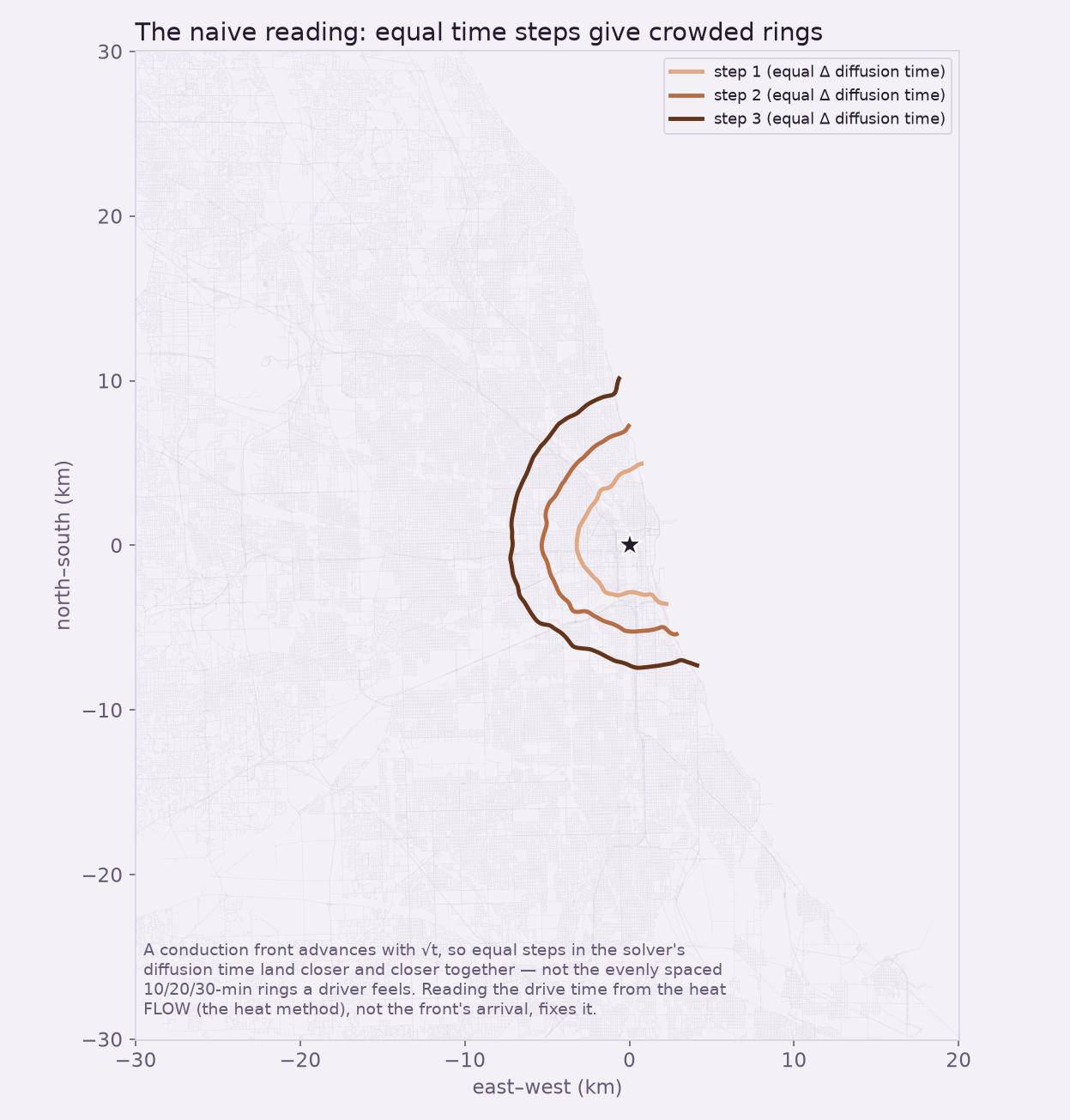
Second — and this one bit harder — a city is not a single road. At every intersection, heat leaks sideways into the cross streets, which soak it up like little reservoirs. On a lone straight road our extraction is essentially exact (we checked it against the textbook closed form and it agreed to 0.16 %). But dropped onto Chicago’s dense grid, that same reading over-states travel time by 47 to 76 %: the front lags because so much heat is busy filling side streets. The shape of the map stays right — the ordering of near and far is faithful — but the clock is badly off. Chasing it into ever-earlier snapshots only walked the error down to 76 %, never close. That is a real limit of the naive analogy, not a bug, and it is exactly why the number needs a better idea.
Reading the drive time from the flow, not the front
The fix is a classical one, the same trick behind the modern “heat method” for measuring distances on shapes. Instead of trusting how hot a point got — the quantity the side-street leakage corrupts — trust only which way the heat is flowing. Right after a pulse of heat is released downtown, the direction of steepest cooling at every intersection points straight back along the fastest route to it. That direction is robust: it stays correct even where the temperature itself has fallen to a billionth of a billionth of its peak.
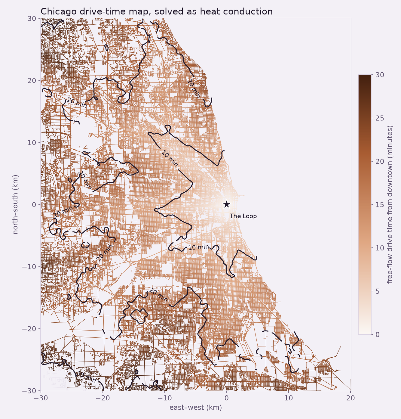
So the map takes two Ansys solves. The first is a transient conduction run: release a unit of heat at the Loop and let it diffuse freely for a short time, giving the flow direction to every one of the 82,375 intersections. A quick arithmetic step turns those directions into a field of unit arrows pointing “away from downtown.” The second solve is a steady conduction problem whose heat sources are exactly that arrow field — and its solved temperature is the drive time, in minutes, at every node. Ansys does both halves; the only thing in between is taking the sign of a difference.
Does it agree with anything real?
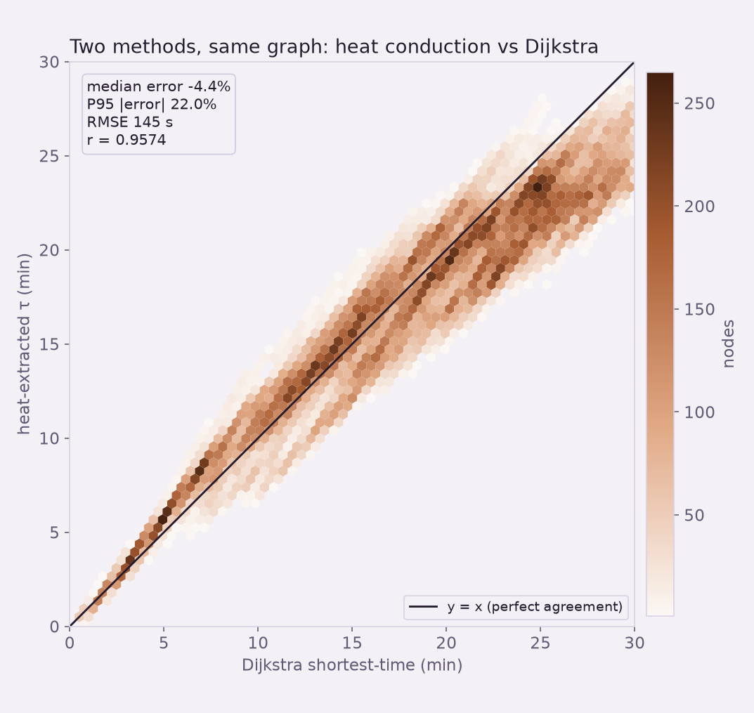
Two independent checks, because a converged solve that is quietly wrong is the default failure mode of this kind of work. The first is a genuinely different algorithm: Dijkstra’s shortest-path search on the identical graph and speeds — a discrete graph computation with nothing diffusive about it. Node for node, the heat-conduction drive times track the shortest-path times to a median 4.4 %, a mean absolute error of 1.9 minutes, and a correlation of 0.957 over 76,009 intersections. The heat solve calls 81,121 nodes reachable within 30 minutes; the shortest-path search calls it 76,185. Two completely different machines, effectively the same map.
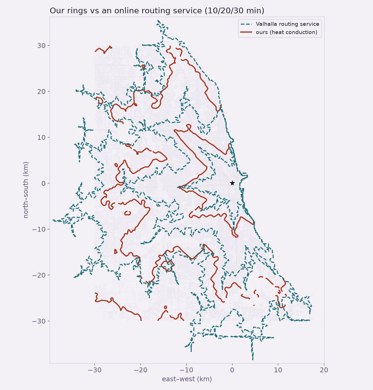
The second check reaches outside our own model entirely: the drive-time rings a live online routing service returns for the same downtown origin. They land in the same neighborhood as ours, with honest, explainable differences — the service reaches a little farther along some highway corridors, where its own speed model and its respect for on-ramps and one-way streets differ from our undirected, speed-limit-only network.
And because it is a real finite-element solve underneath, the solver will draw its own picture of it — the drive-time field on the actual street mesh, straight out of Ansys.
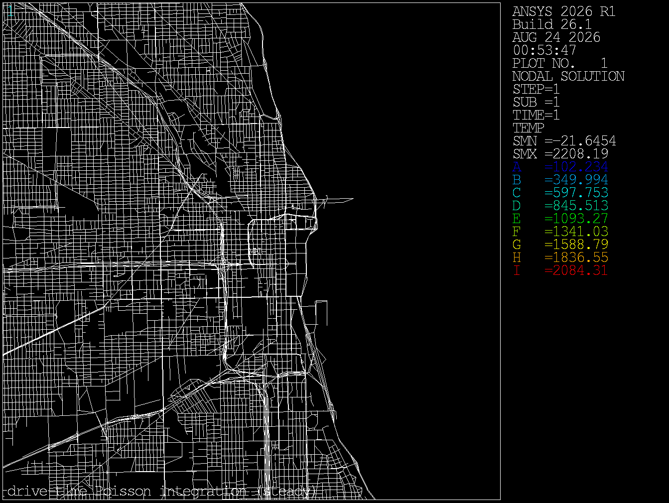
Honest scope. This is a free-flow, speed-limit map, not a promise of door-to-door time. It leaves out traffic (both our map and the routing comparison are free-flow, so the comparison is fair, but real rush-hour rings would be smaller), turn penalties, traffic signals, and stop signs. Conduction is symmetric, so the network is treated as undirected — one-way streets are not modeled, which is the main source of disagreement downtown. Speeds are posted limits where OpenStreetMap tags them and a road-class default otherwise, not measured driving speeds. The domain is clipped to within about 40 free-flow minutes of downtown so the 30-minute ring sits comfortably inside it. The heat method carries a small residual bias (it runs about 4 % fast in the median), reported here rather than tuned away; the naive isotherm reading, by contrast, was 50–80 % off, which is why we did not use it.
Have a problem where the physics itself is the algorithm? Diffusion, potential flow, and conduction turn up as solvers for problems that look nothing like heat — distances on a network, layout and routing, reachability. If you are curious whether an Ansys model could compute something you would not expect it to, we would love to talk it through. Rand Simulation is an Ansys (Synopsys) Apex Channel Partner, and this whole study — geometry, mesh, solve, and post-processing — was run end to end by an agentic AI workflow on our own licenses. Innovation Through Insight™.