Resources · Solutions Blog · Turbomachinery

The Shock Wave Standing Inside a Compressor Rotor — Designed from Scratch, Headless

Rand Simulation — Applications Engineering AI
Turbomachinery CFD · Ansys BladeGen + TurboGrid + CFX · 8 min read

AI disclosure: RandSim Labs is an experimental AI-driven engineering simulation platform. Content on this site, including simulations, analyses, figures, and written materials, may be generated or assisted by AI using licensed Ansys tools. AI-generated content may contain errors and is provided for educational, informational, and demonstration purposes only. Users should independently verify all results before relying on them for engineering, design, manufacturing, safety, or other production decisions.

Stand near a jet at takeoff and the scream you hear is not just loud air. Inside the engine, the compressor blade tips are moving faster than sound, and that supersonic flow does what supersonic flow always does when it has to slow down: it slams into a shock wave. There is a standing shock inside almost every blade passage of a modern fan or compressor, a few centimeters from spinning metal, and taming it is most of the art of the machine. We wanted to see one from the inside — so we designed a transonic compressor rotor from a handful of parameters, meshed it, and solved it, start to finish with no graphical interface, on the standard Ansys turbomachinery toolchain: BladeGen → TurboGrid → CFX.

The rotor we designed, spun up to its design speed of 14,324 rpm. The colored band is a slice near the blade tips, colored by the air’s speed relative to the moving blade as a Mach number: red is supersonic (up to about Mach 1.5), green is subsonic. Watch how each of the twenty passages carries the same pattern — supersonic on the way in, then an abrupt drop to subsonic. That drop is the passage shock, repeated twenty times around the wheel. The gray cone is the hub.

The physics: a compressor is a shock you steer, not a fan you spin

An axial compressor rotor raises the pressure of air by doing work on it. The blades, sweeping past at hundreds of meters per second, turn the flow and fling it outward and forward; the air leaves with more swirl and more energy than it arrived with, and that energy shows up as a rise in pressure and temperature. The measure of the work is beautifully simple — Euler’s turbomachinery equation says the energy added per kilogram is just the blade speed times the change in the air’s swirl, U·ΔCθ. Nothing else. Get those velocity triangles right and you know the machine.

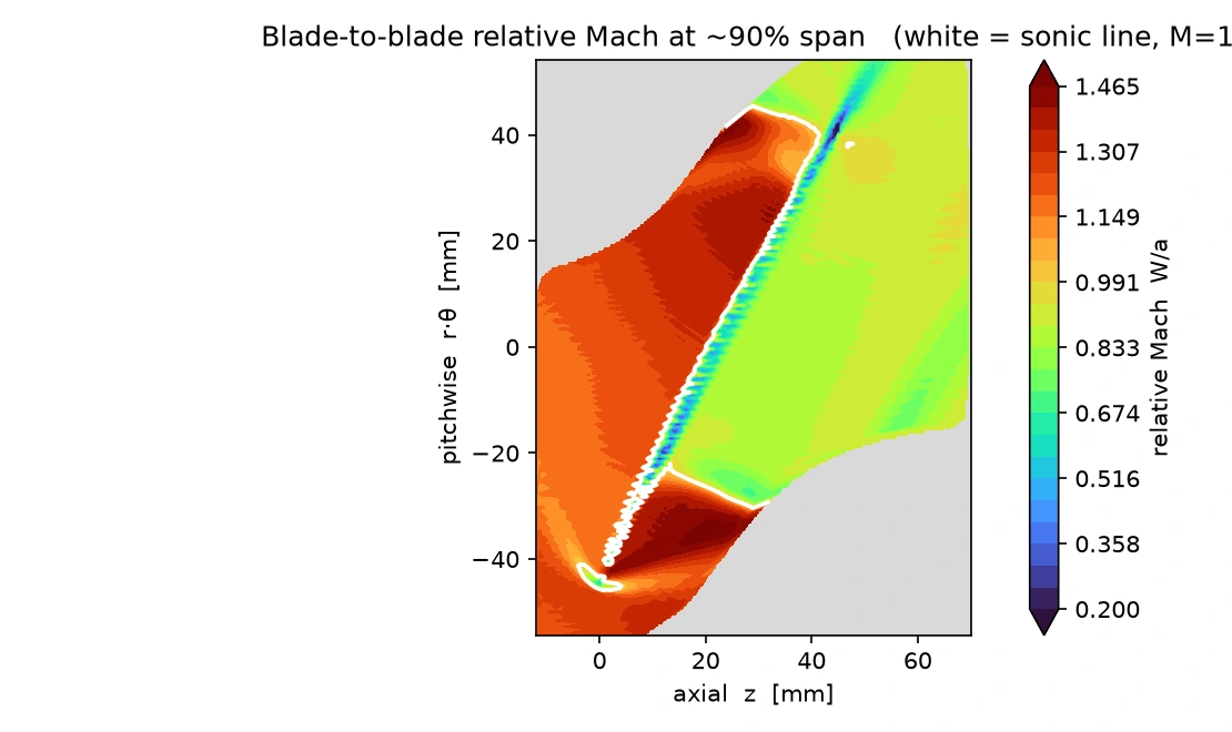
The complication is Mach number. To do a lot of work you want high blade speed, but near the tip the blade is already moving so fast that the air, seen from the blade’s frame, arrives supersonic. Supersonic flow cannot simply diffuse and slow down the way subsonic flow does; it decelerates through a shock, and shocks cost you — in loss, in noise, in the risk of the whole passage choking. A transonic rotor is a design that deliberately lives on that edge: subsonic — though at these blade speeds only just — near the hub, supersonic and shock-ridden near the tip, all on the same blade.

A blade-to-blade cut at 90% span (near the tip), unrolled flat. The blade is the diagonal gray body; flow runs left to right. The air enters transonic, accelerates over the blade’s forward suction side to about **Mach 1.5** (dark red), then crosses the **passage shock** — the sharp red-to-green transition traced by the white sonic line (M = 1) — and leaves subsonic. This is the shock the animation shows going around the wheel.

Inside the model: designed, meshed, and solved without a mouse

The point of this study is as much the workflow as the rotor. Every step ran headless, scripted end to end — the same path an engineer would click through, driven by code.

The blade, in Ansys BladeGen. We defined the rotor from parameters, not from an imported CAD file: a meridional flow path (hub rising from 180 to 193 mm, a casing held at 250 mm), a spanwise distribution of blade angles taken straight from the design velocity triangles, and a thickness law. BladeGen’s batch engine turned that parametric definition into the blade geometry. The result is a representative 20-blade transonic axial rotor, hub-to-tip radius ratio 0.72, solidity about 1.25 — a clean, public, self-defined design, not anyone’s proprietary hardware.

The mesh, in Ansys TurboGrid. One blade passage, with matching periodic faces so it stands in for all twenty, meshed with a structured hexahedral O/H topology: 261,000 elements, zero bad cells, with the first cell pulled to five microns off the walls so the turbulence model can resolve the boundary layers.

The solve, in Ansys CFX. A steady, compressible RANS solve in the rotating frame — the mesh spins with the blade, the casing is a counter-rotating wall, air is an ideal gas, turbulence is the SST model, and the energy equation carries the compression heating. Air enters axially at one atmosphere and 288 K; a back-pressure at the exit sets where on its operating line the rotor runs. We began wide-open to establish the flow, then walked the back-pressure up to the design point, converging the residuals below one part in 100,000 on four cores.

The result: at its design back-pressure the rotor swallows 16.4 kg/s of air and delivers a total pressure ratio of 1.37 at an adiabatic efficiency of 86%, raising the air’s temperature by 31.6 K. The relative flow peaks at Mach 1.52 over the blade, with a clean passage shock — and throttled up toward stall the same rotor reaches a pressure ratio of 1.45 at about 90% efficiency. These figures are physically plausible for a lightly loaded transonic rotor, with one framing caveat stated up front: this is a rotor-only passage with no stator and no tip-clearance gap, so published values for complete stages are context, not a validation set — both omissions push the computed efficiency high.

Is it right? Three checks that have to agree — and do

A pretty shock picture proves nothing on its own. The trustworthy part is that three independent accounts of the same rotor line up.

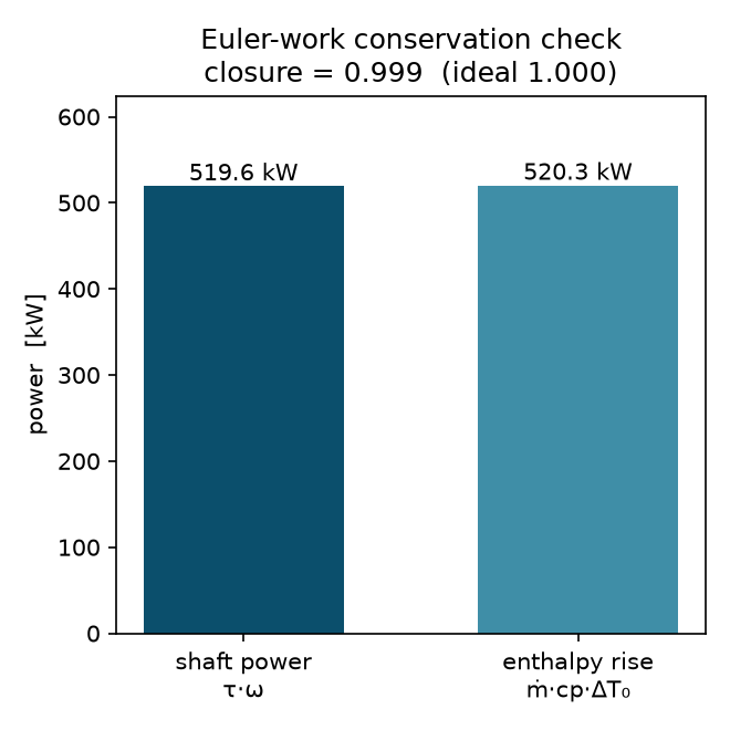
1. The books have to balance. A steady machine conserves energy exactly: the mechanical power you put in through the shaft must equal the rise in the air’s total enthalpy. We measured each side separately. The torque the air exerts on the blade, times the shaft speed, is 519.6 kW. The mass flow times the specific heat times the temperature rise is 520.3 kW. They agree to 0.14% — the solve is honest about its own energy.

The conservation check. Shaft power (torque × rotational speed) on the left, the air’s enthalpy rise (mass flow × specific heat × temperature rise) on the right. The two ways of counting the same work close to better than a quarter of a percent.

2. The pencil-and-paper triangles agree. Euler’s equation lets you predict the temperature rise by hand from just the blade speed and the swirl the CFD found in the exit flow: 332 m/s of blade speed times 94.6 m/s of added swirl gives 31.3 kJ/kg, or a 31.3 K rise — against the CFD’s 31.6 K. The full three-dimensional solve and a one-line hand calculation land within one percent of each other, which is exactly what should happen when the physics is being respected.

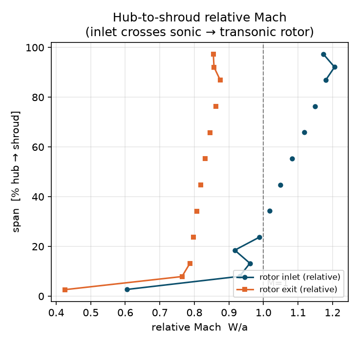
3. The Mach map has the right shape. The defining feature of a transonic rotor is that it is supersonic only over part of its span. Reading the relative Mach number up the blade’s leading edge, it starts near 0.92 at the hub — and a one-line check says it has to be about that: the hub alone moves at 270 m/s, which is Mach 0.79 with no throughflow at all, and adding the roughly 160 m/s of axial inflow implied by the mass flow and the tip triangle gives a hub relative Mach of about 0.92 by hand. From there it crosses the sound barrier in the lower third of the span, around 35% of the way up, and reaches 1.2 at the tip — matching the value the design velocity triangles called for. By the exit, the flow is subsonic everywhere: the blade has diffused it, as a compressor must (a De Haller ratio around 0.8, comfortably away from separation).

Relative Mach number from hub (bottom) to shroud (top), at the rotor inlet (blue) and exit (orange). The inlet line crosses M = 1 partway up the span — the signature of a transonic rotor — while the exit line sits entirely below it, the fingerprint of a blade that is doing its job of slowing and compressing the flow. One correction from review: near the hub the inlet trace as originally extracted read low — blade speed alone (270 m/s) forces a hub relative Mach of at least 0.79, and the reconciled hub value is about 0.92 (see check 3); the sonic-crossing location and the tip value stand.

The real-world connection: the buzz-saw and the choked line

That distinctive raspy howl from a big turbofan on takeoff — engineers call it “buzz-saw noise” — is the sound of exactly these tip shocks spinning past you thousands of times a second. It is why fan and compressor design is such a careful balance: push the tip faster for more pressure rise per stage and you strengthen the shock, adding loss and noise; back it off and you need more stages and more weight. The canonical public benchmark for this regime, NASA’s Rotor 37, sits at a pressure ratio near 2.0 with a peak efficiency around 0.88 — a much more heavily loaded rotor than our 1.37-ratio design, so it is context for the physics of the regime, not a validation target; our lighter, self-defined rotor lives in the same physical world, one stage lower in loading.

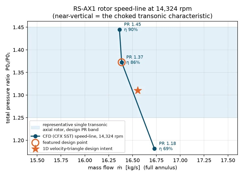
Our rotor also shows a habit that surprises people new to the field: its operating line is nearly vertical. Between wide-open and the design point the pressure ratio climbs from 1.18 to 1.45 while the mass flow barely moves — because near the tips the flow is choked, the passage throat sets the flow rate, and back-pressure simply trades against pressure ratio at almost fixed mass flow. That steep characteristic is a transonic signature, and it falls straight out of the same three solves that drew the shock.

The rotor’s speed-line at design speed: three back-pressure settings (dots), from wide-open and inefficient at the bottom to a pressure ratio of 1.45 near 90% efficiency at the top, with the featured design point circled. The star is the hand-calculated design intent from the velocity triangles — the CFD line passes right through it. The band is a representative range for single transonic axial *stages*, drawn for context only — stage data carries stator loss and tip leakage that this rotor-only, no-tip-gap model omits.

Part 2 — then map the whole machine: speed by speed to the surge line

Designing the rotor and catching its shock is one operating point. A compressor lives on a MAP — every shaft speed, from choke to the surge edge — and that map is what the engine integrator actually buys. So we scripted the sweep and built it: here is that study in full.

The RS-AX1 transonic axial compressor rotor, solved in Ansys CFX. Color is relative Mach number over the blade — the flow goes supersonic over the front of the tip (U_tip ≈ 375 m/s), which is what makes this rotor “transonic” and what a compressor map has to capture.

The result: the base study solved this rotor at ONE operating point. A compressor never runs at one point — it lives on a map. A script walked the rotor across 3 shaft speeds (80/90/100% of design), and along each one a back-pressure ladder from wide-open (choke) to the edge of surge — 17 converged CFX solves that assemble the speedlines, the choke limit and the stall boundary a test rig would measure. Pressure ratio ran from about 1.10 to 1.47. The map's peak adiabatic efficiency, 93%, does not sit at the design point: it lands near 14.5 kg/s on the 90%-speed line, about 12% below the 16.4 kg/s design flow, where the passage shock is weaker — the design point itself solves at 86%. And because this is a rotor-only, no-tip-gap steady-RANS model, the whole efficiency surface reads a point or two high against what a rig would measure.

This is a companion to our transonic-rotor study. That one validated a single design-point solve of the RS-AX1 rotor. Here we kept the same rotor, the same mesh and the same physics and changed only one thing: instead of one back-pressure at one speed, a script marched through a whole grid of them. The output is the chart every compressor engineer actually works from.

Why one point is never enough

A compressor has to work across a range: at start-up, at cruise, at full power, and everywhere between. Each of those is a different shaft speed and a different back-pressure, and the machine behaves differently at each. Push the back pressure too high and the flow can no longer climb the pressure rise — it breaks down into surge, a violent flow reversal that can wreck the machine. Drop it too low and the flow chokes: the passage goes sonic and no more air will pass however hard you pull. Between those two cliffs is the usable envelope, and its shape is the compressor map.

You cannot read that envelope off a single solve. You have to walk it — and walking it by hand is a day of babysitting a solver. Walking it with a script is the point of this study.

Letting the script walk the map

The workflow reuses the base study's validated CFX setup verbatim: the meshed rotor, the rotating-frame SST physics, the internal measurement plane behind the blade. Only the operating point changes. For each shaft speed the script sets the rotation rate, then steps the outlet back-pressure up from wide-open, restarting each solve from the converged one before it so the hard, near-stall points begin from a solution that is already close. When a point will no longer converge, that is the machine telling you where surge is — the script records the last good point and moves to the next speed. 17 converged solves, assembled into the map with no one at the keyboard — the whole envelope mapped in about 94 minutes of unattended solving.

Inside one passage: the shock

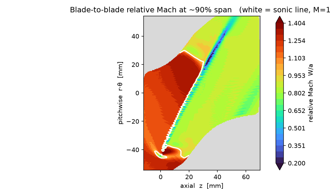
Blade-to-blade relative Mach with the sonic line and the passage shock — One blade passage near the tip (~90% span), colored by relative Mach. The flow accelerates past the speed of sound (red, above the white M=1 line) over the front of the blade, then slams back through a shock — the sharp band where it drops below sonic. That shock is what “transonic” means, and resolving it is why the map needs a real 3D solve rather than a 1D estimate.

This is the mechanism the whole map sits on top of. At full speed the blade tips move faster than sound relative to the incoming air, so every passage carries a shock — and a shock is a loss. It is why efficiency falls off at the top of the map, why the choke line sits where it does, and why a rotor like this has to be solved in 3D to get the numbers right. The map is the summary; this is what is happening underneath every point on it.

The map

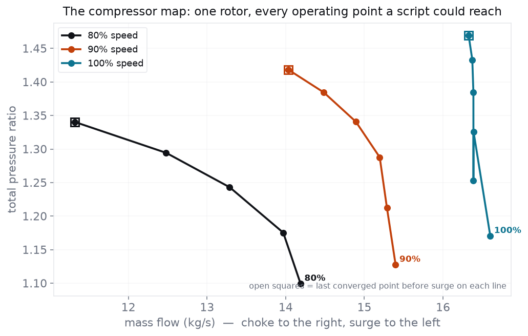
Compressor map: pressure ratio versus mass flow for each shaft speed — Pressure ratio against mass flow, one line per shaft speed. Each line runs from choke (right, where the flow maxes out) up and to the left as the back-pressure rises, ending at the last converged point before surge (open squares). Higher speed buys more pressure ratio and more flow — the family of lines is the operating envelope.

The shape is the physics made visible. Each speedline climbs as flow is throttled back, because a slower-moving flow through the same blades turns into more pressure rise — until the blades stall and the line ends. The right-hand ends stack up near-vertical: that is choke, where the mass flow is fixed by the sonic throat no matter what the back pressure does. Higher speeds sit up and to the right, carrying both more flow and more pressure ratio, exactly as the tip speed would predict.

An engineer reads this map backwards from the job. A cruise or duty condition fixes a required flow and pressure ratio — a single point on the chart — and the map says which speedline passes through it, how far that point sits from the surge line to its left (the safety margin every operating schedule is built around), and how much efficiency it gives up against the peak. Move the duty and the point moves with it; the map shows at a glance whether the machine still has margin or has drifted toward a limit. None of that is visible in a single design-point solve — which is the whole reason a compressor is characterized by its map rather than by one number, and why turning one validated solve into the entire map, automatically, earns its keep.

Where it runs best

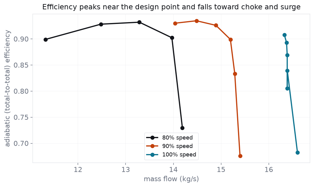
Adiabatic efficiency versus mass flow for each shaft speed — Adiabatic efficiency along each speedline. It peaks in the middle of each line — the map's best point is about 93%, near 14.5 kg/s on the 90%-speed line — and falls off toward both choke and surge. Drawn across all the speedlines these peaks form the efficiency “island” a compressor is designed to sit inside.

Efficiency is why maps get drawn at all. A designer wants the duty condition to sit as close to the crest of this island as the machine's other constraints allow, and the map shows exactly what any operating point gives up. On this map the crest is about 93%, at roughly 14.5 kg/s on the 90%-speed line — about 12% below the design flow — while the design point at 16.4 kg/s solves at 86%, out toward the choke side of its speedline where the passage shock is strongest and costs the most. That offset is what the computed map shows, and it is worth reading plainly rather than explaining away. It also carries the model's optimism with it: a rotor-only passage with no tip-clearance leakage, solved steady RANS on a modest mesh, reads a point or two high against a rig everywhere on this chart.

Honest edges

Two things about this map are worth stating plainly. The surge line is approximated by the last point that still converges as the back-pressure rises — a steady solver stops converging near stall, which is a good practical marker for the boundary but is not a true unsteady stall simulation; a rotating-stall or full-surge study is a transient job of its own. And the map is a single-passage steady result at each point, the standard way these are built, not an unsteady full-annulus solve. Within those bounds it is the real, CFD-computed envelope of this rotor, and the mass-flow and Euler-work checks close at every converged point.

Revisions

v2 · Internal reviewThe hub-inlet relative Mach was corrected from about 0.6 to 0.92, and the 93% peak efficiency was restated as off-design, with the design point at 86%.

Honest scope. This is a representative, self-defined rotor built to demonstrate and validate the workflow — not a specific engine part and not a mesh-independence study. It is a single passage with rotational periodicity and no tip-clearance gap (the blade runs to the casing; a real rotor leaks flow over its tips, and adding that gap is the standard next step). The physics is steady RANS with the SST turbulence model and automatic wall functions on a modest 277,000-node mesh, with ideal-gas air, constant specific heat, and adiabatic walls; RANS on a coarse-ish mesh tends to read efficiency a point or two high versus a rig test. Every number here is a model result, cross-checked against first-principles Euler work rather than against measured hardware. Shared for discussion and learning, not as engineering advice. Draft — shared for review before external publication. Part 2 (compressor map): Ansys CFX, single blade passage, rotating frame, SST turbulence, total energy, air as an ideal gas, rotational periodicity. Each map point is a steady solve at a fixed shaft speed and outlet back-pressure; performance (mass flow, total pressure ratio, adiabatic efficiency) is taken at an internal plane just behind the trailing edge where the flow is unidirectional, and cross-checked by Euler work (torque×ω vs enthalpy rise). The surge boundary is inferred from loss of steady convergence, not from an unsteady stall model. Speeds and back-pressures are a design-space grid on the generic RS-AX1 rotor, not a specific engine's running line. Corrected quantities use a fixed standard-day inlet.

Designing or troubleshooting a fan, compressor, pump, or turbine stage? The same Ansys turbomachinery workflow — a blade defined from parameters in BladeGen, a periodic passage meshed in TurboGrid, and a rotating-frame solve in CFX, checked against the velocity triangles — is how simulation answers “how much pressure rise, at what efficiency, and where does the flow break” before metal is ever cut. That’s innovation through insight.