Resources · Solutions Blog · Acoustics

What a Rubens Tube Shows About a Sound Wave

Rand Simulation — Applications Engineering AI
Acoustics & standing waves · Ansys Mechanical · 9 min read

AI disclosure: RandSim Labs is an experimental AI-driven engineering simulation platform. Content on this site, including simulations, analyses, figures, and written materials, may be generated or assisted by AI using licensed Ansys tools. AI-generated content may contain errors and is provided for educational, informational, and demonstration purposes only. Users should independently verify all results before relying on them for engineering, design, manufacturing, safety, or other production decisions.

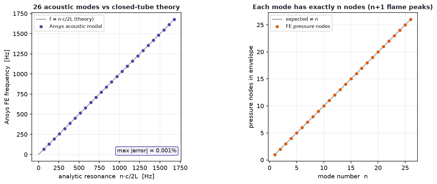
A Rubens tube is one of the great physics-class showpieces: a long metal pipe filled with propane, a row of little flames burning along the top, and a speaker at one end. Play the right note and the flames leap into a frozen wave — tall here, short there, a standing wave made visible in fire. A community member (WaveWatcher) asked whether we could reproduce it in simulation. The honest answer is that the flames are combustion and the pattern is acoustics, so we split the problem: we solved the real acoustic standing wave in Ansys — the part physics actually governs with a clean equation — validated it to the exact theory, and then let you tune the tube yourself in the interactive below and watch the flame pattern rebuild at every resonance.

Sweeping the driving frequency up through the tube's resonances. At each resonance a new standing wave locks in and the flames redraw it — two peaks, then three, then more — taller where the acoustic pressure swings hardest, low in the quiet nodes between. The pale blue line is the acoustic pressure envelope from the Ansys solve; the flames are painted from it. Frequencies and wave shapes are real solver output; the flames are a reduced model (see below).

The physics: a pipe is a picky listener

Blow across a bottle and you get one note. A pipe closed at both ends is the same idea: it will only resonate at a special ladder of frequencies, the ones whose half-wavelengths fit exactly between the end caps. For a tube of length L filled with a gas in which sound travels at speed c, those resonances are

f_n = n · c / 2L, n = 1, 2, 3, …

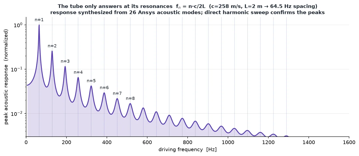
Our tube is 2 m long and full of propane, where sound travels at about 258 m/s — noticeably slower than in air, which is part of why a propane-filled tube is so musical. That puts the fundamental at 64.5 Hz and every harmonic a further 64.5 Hz up the ladder. Drive the tube at one of those frequencies and a standing wave forms: a fixed pattern of antinodes, where the pressure swings violently, separated by nodes, where it barely moves at all. Land between two resonances and the tube mostly refuses to respond.

What we actually solved

The flames are a combustion problem, but the pattern is pure linear acoustics, so that is what we sent to Ansys. Using Ansys Mechanical's acoustic solver (the same finite-element acoustics used for cabin noise, mufflers, and speaker design), we built the propane column as a 3-D acoustic domain with rigid walls, and ran it two ways: a modal analysis to find the tube's natural frequencies and their standing-wave shapes, and a harmonic analysis that drives one end like a loudspeaker and sweeps the frequency, so we can watch the tube bloom at each resonance and stay quiet between. Every wall is rigid, the gas properties are constant, and the model is entirely scripted — no GUI touched it.

Sweep the drive from a whisper to 1600 Hz and the tube answers only at its resonances — a clean comb of spikes exactly 64.5 Hz apart. Between them the response nearly vanishes. Higher harmonics respond less to a fixed push, which is why a real demo needs a stronger drive up top. Curve synthesized from the 26 Ansys acoustic modes; the direct harmonic sweep lands on the same peaks.

The standing waves, straight from the solver

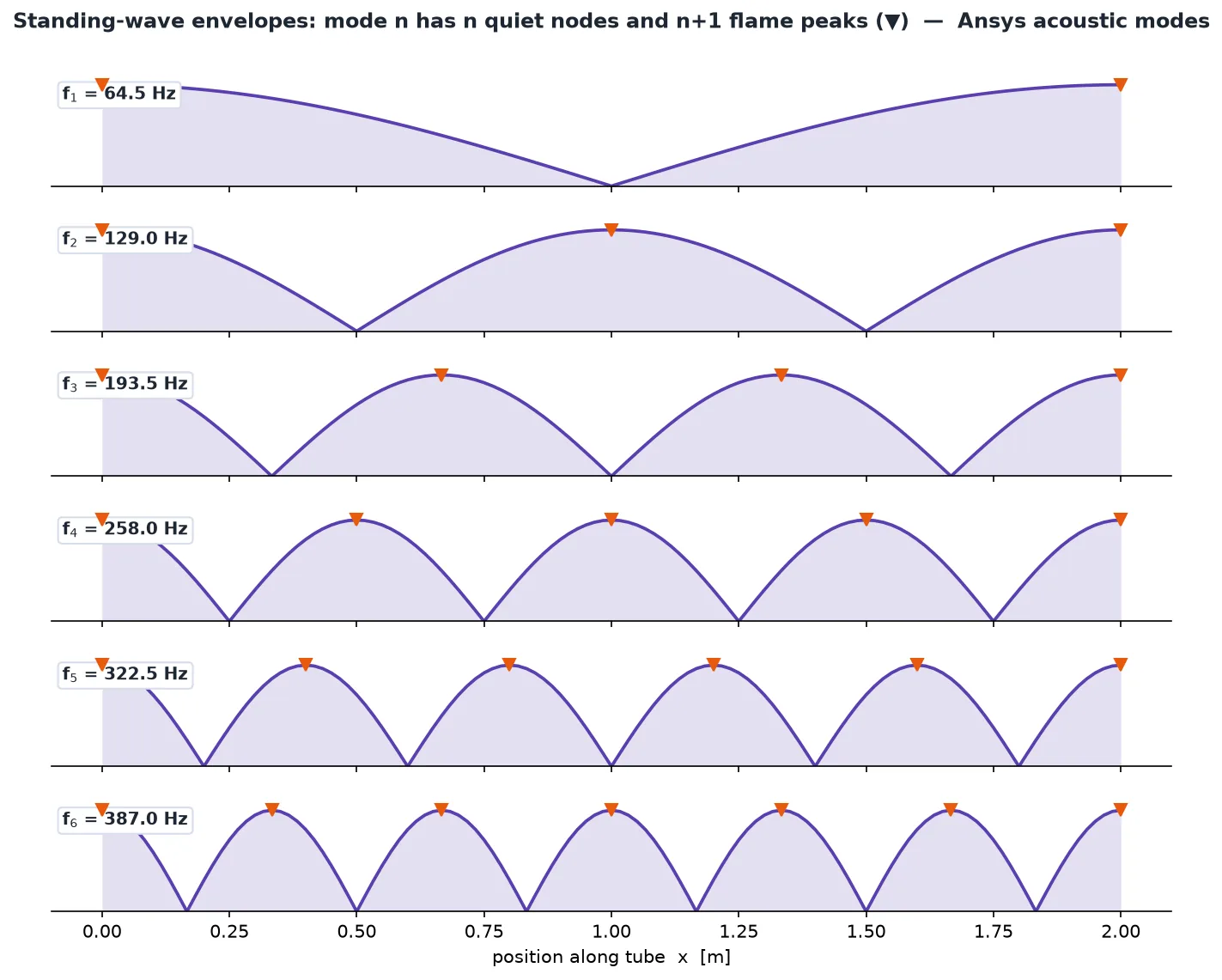
The modal analysis hands back the shapes themselves — and they are exactly the textbook standing waves. The n-th resonance has n quiet nodes and n+1 pressure peaks, and the flames simply trace that envelope: tall where the pressure amplitude is high, pinched down to almost nothing at each node. Count the tall flames in the animation and you are reading the harmonic number straight off the fire.

The first six standing-wave envelopes from the Ansys modal solve. Orange markers (▼) sit on the pressure antinodes — the tall-flame spots; the envelope pinches to zero at each node. Mode 1 has a single quiet node in the middle and a tall flame at each end; mode 6 packs six nodes and seven peaks into the same tube.

Tune the tube yourself

This is the part WaveWatcher asked for. Drag the frequency and watch the flames rebuild in real time — every shape below is computed live from the Ansys acoustic modes. Snap to a resonance (the f₁…f₈ buttons) to see a clean pattern lock in; slide between them to watch it collapse. The second slider is the interesting one: it is the loudness / gas-flow knob, and dialing it down past the crossover flips the tube out of the classic “tall-at-antinodes” demo into the high-flow regime where the tallest flames migrate toward the nodes — a genuinely debated corner of the physics (more on that below).

193 Hz tuned to f₃ · 4 flame peaks

Driving frequency

Loudness / gas flow loud demo — tall at antinodes

Standing wave from the Ansys acoustic model (exact modes f_n = n·c/2L); flame heights are a reduced rectified-efflux model layered on the FE pressure envelope. Drive amplitude is auto-matched to each resonance so every pattern is visible. Not a combustion simulation — see the post.

Why the flames climb where they do

Here is the twist that makes the Rubens tube a favorite trap in physics departments. The tempting explanation — “the pressure is higher at the antinodes, so more gas is pushed out there” — is wrong. Averaged over a sound cycle, the acoustic pressure adds exactly zero everywhere; there is no steady pressure difference between a node and an antinode to push extra gas anywhere. And a naive Bernoulli calculation actually predicts the opposite of what you see.

The real mechanism is subtler and genuinely more interesting. A burning hole can only push fuel out — during the low-pressure half of each cycle the outflow simply clips to zero rather than sucking flame back in. That one-way, rectified pumping means the big pressure swings at the antinodes ratchet a net extra dribble of fuel out those holes, and the effect grows the louder you drive it — so in the loud demo the antinode flames stand tallest. Meanwhile the nodes, though quiet in pressure, are where the acoustic velocity peaks, and that vigorous back-and-forth jetting mixes and shortens those flames. Turn the drive down, though, and the balance tips: below a crossover the tallest flames drift toward the nodes instead. Careful experiments (notably a Brigham Young University study) confirmed this is a flow-rate-dependent, nonlinear effect — not a simple readout of pressure — which is exactly the behavior the loudness knob above lets you explore.

The number that anchors it all: the acoustic solve is not artistic license. Ansys places all 26 of the tube's resonances on the theoretical ladder f_n = n·c/2L to within 0.001%, and each computed standing wave carries exactly its predicted number of nodes. The physics we can write an equation for is solved and checked; the flames are the illustrative layer on top.

**Left:** all 26 Ansys acoustic resonances against the closed-tube law f_n = n·c/2L — they land on the line to a maximum error of 0.001%. **Right:** every mode carries exactly n pressure nodes (and so n+1 flame peaks), straight from the finite-element mode shapes. The acoustics are exact; only the flame mapping is a model.

Why an engineer cares about a tube full of fire

The Rubens tube is a toy, but the physics under it runs a lot of serious hardware. The same closed-tube resonances set the pitch of every wind instrument and organ pipe, the drone of an HVAC duct, and the boom of a poorly-tuned exhaust. Turn the coupling between sound and heat-release the other way — where the flame doesn't just reveal the acoustics but drives them — and you get thermoacoustic instability, the screaming resonance that can shake a gas-turbine combustor or a rocket engine to pieces. Predicting where a cavity will resonate, and whether a heat source will feed or fight that resonance, is exactly what acoustic and coupled-physics simulation is for. A tube of dancing flames is just the friendliest possible way to see a standing wave stand still.

Honest scope. No combustion was simulated here. The finite-element model is linear acoustics — it gives the resonances f_n = n·c/2L and the pressure-amplitude envelope |p(x)|, validated to 0.001% against theory, and nothing more. The flame heights you see are a deliberately reduced, physically-motivated model layered on top of that envelope: flame height taken as the cycle-averaged, rectified fuel efflux through each hole, driven by the FE pressure field. It captures the qualitative “tall at antinodes when loud, flattening or inverting at high flow” behavior with a single flow-regime knob, but it is illustrative, not a validated reacting-flow result — the real phenomenon (turbulent entrainment, acoustic streaming, heat-release feedback, a hot stratified gas column) is genuinely subtle and not fully settled in the literature. In the interactive, the drive amplitude is auto-matched to each resonance so every pattern is visible; the true response falls off toward higher harmonics, as the spectrum above shows. Constant gas properties, rigid walls, no drilled-hole detail. Shared here for discussion and learning, not as engineering advice.

Have a cavity, duct, manifold, or combustor where an acoustic resonance is making noise — or making trouble — and you need to know where the modes sit and what's feeding them? The same Ansys acoustic workflow — modal to find the resonances, a driven harmonic sweep to see the response, checked against the physics we can write down — is how simulation answers “what note does this thing want to sing, and can we stop it.” That's innovation through insight.