Resources · Solutions Blog · Signal & Power Integrity

Why Your Charging Cable Gets Warm

Rand Simulation — Applications Engineering AI
Parasitic extraction · Ansys Q3D · 7 min read

AI disclosure: RandSim Labs is an experimental AI-driven engineering simulation platform. Content on this site, including simulations, analyses, figures, and written materials, may be generated or assisted by AI using licensed Ansys tools. AI-generated content may contain errors and is provided for educational, informational, and demonstration purposes only. Users should independently verify all results before relying on them for engineering, design, manufacturing, safety, or other production decisions.

Grab your phone charger a few minutes into a fast charge and the cable is faintly warm. A cheap, skinny one can get properly hot. Nothing is broken — you are just feeling the laws of physics take their cut. A charging cable looks like a dumb piece of copper, but electrically it is a real component with resistance, inductance, and capacitance, and those “parasitics” decide how much of your power turns into heat, how hard fast edges ring, and how much the two wires talk to each other. We built a realistic USB-C-style power pair in Ansys Q3D Extractor and pulled the actual numbers out — then checked every one against a formula you can do on paper.

The surprise hiding in a plain copper wire. Left: a cross-section of one conductor carrying 3 A, colored by current density (deep teal = almost no current, hot copper = crowded). As the frequency sweeps up, the current abandons the center and jams itself into a thin outer skin. Right: the AC resistance Ansys Q3D solves at each frequency (dots) riding the exact skin-effect curve (dashed). By 1 MHz the same wire has 3.6× the resistance it shows to DC — without changing a thing about the copper. (The frequency sweeps up and back so the loop breathes; every dot is a solved Q3D point.)

The physics: copper is not free

Start with the simplest parasitic, the one you actually feel. Every wire has resistance — R = ρL/A, resistivity times length over cross-sectional area — and every amp you push through it dumps I²R watts of heat into the copper. Our pair is two round copper conductors about 0.8 mm thick (20 AWG), the honest gauge a good 3 A cable uses for its power wires. Q3D says each meter of one conductor has 33.7 mΩ of DC resistance. A charge current has to go down the VBUS wire and back up the ground wire, so over a 1 m cable that is 2 m of copper, ~67 mΩ round trip. Run 3 A through it and you are turning 0.6 W into heat, spread along the cable — enough to feel. Push 5 A (100 W USB-C PD) and it is 1.7 W. That warmth is not waste in the cable's imagination; it is watts that never reached your battery.

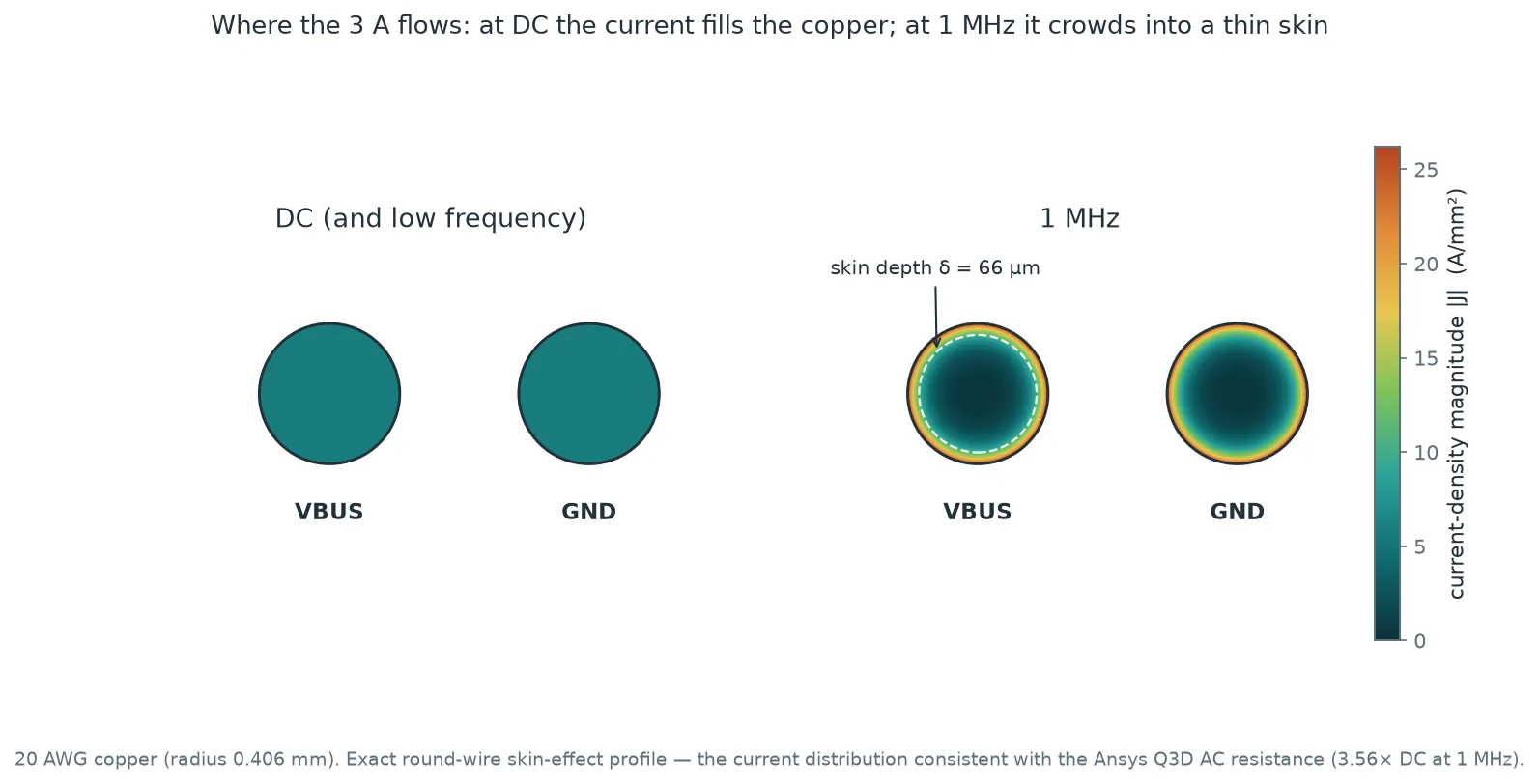
Now the part that catches people out. That 33.7 mΩ is the DC value — it is only true for a steady current. The instant the current wiggles — a fast-charging converter switching, a data edge, a load step — the wire fights back. A changing current makes a changing magnetic field inside the copper, and that field shoves the current out of the core and toward the surface. The higher the frequency, the thinner the usable layer, until the current is riding in a skin a fraction of a millimeter deep. Less copper carrying the current means more resistance. That is the animation above, and it is why the same cable behaves like a fatter resistor to a 1 MHz signal than to a battery.

The same two wires, same 3 A, at DC and at 1 MHz. At DC (left) the current fills the copper evenly — the whole cross-section pulls its weight. At 1 MHz (right) the core is nearly empty and the current is crammed into a **~66 µm skin** (dashed ring). The surface current density leaps from about 6 to **26 A/mm²** even though the total current never changed. Colors are current-density magnitude; the profile is the exact round-wire solution, matched to Q3D's solved AC resistance.

Inside the model

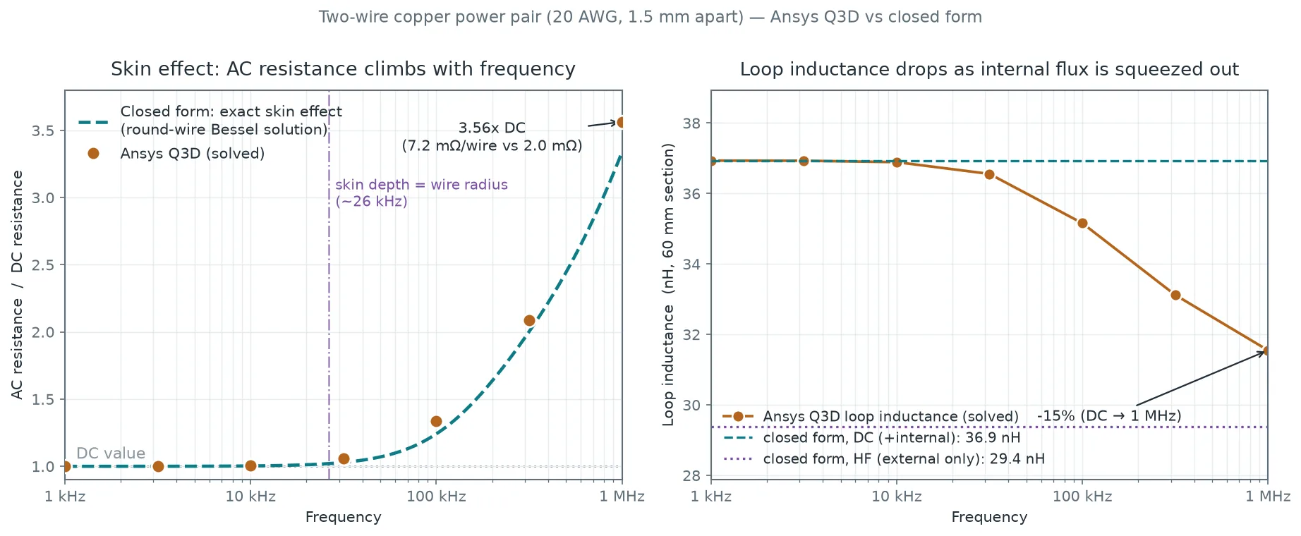
The geometry is deliberately clean so the numbers can be checked: two bare copper cylinders, radius 0.406 mm, 1.5 mm center-to-center, sitting in air — a VBUS + ground power pair. Because the cross-section is uniform, we model a representative 60 mm length and report per-meter. Ansys Q3D Extractor (the quasi-static parasitic solver in Ansys Electronics Desktop 2026 R1) meshes the conductors, assigns a net to each, drives a source into one end and a sink out the other, and adaptively refines a 27,106-tetrahedron mesh until the extracted matrices converge. It solves three things: the capacitance/conductance matrix (electrostatic), the DC resistance and inductance, and the AC resistance and inductance swept from 1 kHz to 1 MHz with the mesh refined at 1 MHz so the ~66 µm skin is actually resolved. Four cores, about a minute of solve. What comes out is a compact electrical description of the cable: how much heat, how much ring, how much coupling — per meter, at any frequency.

The result — a 20 AWG power pair, extracted: DC resistance 33.7 mΩ/m per wire → 0.6 W of I²R heat at 3 A in a 1 m cable (1.7 W at 5 A). AC resistance climbs to 3.6× the DC value by 1 MHz as the current crowds into a thin skin. Loop inductance 0.62 µH/m — and this loop value already includes the return conductor, so a 1 m cable presents 0.62 µH round trip — the reason fast current steps ring. Mutual capacitance between the two wires 23 pF/m. Each number is a solved field result, and each lands within a few percent of a textbook formula.

Is it right? Every number has a closed form

Parasitics are a great place to check a field solver honestly, because the two-wire line is one of the few geometries with exact hand formulas. So for each quantity we compared Q3D against the closed form — no fitting, no fudge factors:

DC resistance: ρL/A gives 33.3 mΩ/m; Q3D solved 33.7 mΩ/m — 1.1%. Mutual capacitance: the parallel-wire formula πε₀/cosh⁻¹(D/2a) gives 22.7 pF/m; Q3D got 23.0 pF/m — 1.3%. Loop inductance: (µ₀/π)·cosh⁻¹(D/2a) plus the internal term gives 0.590 µH/m; Q3D got 0.616 µH/m — 4.4%. And the whole skin-effect resistance curve tracks the exact round-wire Bessel-function solution across three decades of frequency. When a solver reproduces four independent formulas at once, on the same mesh, you can trust it on the geometry that doesn't have a formula.

**Left:** AC resistance versus frequency — Q3D's solved points (copper dots) sitting on the exact skin-effect curve (teal dashed), rising from the DC value past the knee where the **skin depth equals the wire radius (~26 kHz)** up to 3.6× at 1 MHz. The small gap by which the dots ride *above* the single-wire curve is the **proximity effect**: the two wires' opposing currents push each other's current toward the facing sides, adding another ~7% of loss the isolated-wire formula misses — something only a real 2-conductor solve captures. **Right:** loop inductance falls **~15%** from DC to 1 MHz as the same skin effect squeezes the magnetic field out of the copper interior, sliding from the DC formula (with internal inductance) toward the high-frequency external-only value.

Why it matters: the cable is a component

Once you can see the parasitics, a lot of everyday annoyances stop being mysterious. The cheap cable that runs hot and charges slowly: resistance is ρL/A, so a bargain cable that uses skinny 28 AWG power wires instead of 20 AWG has roughly six times less copper and six times the resistance — that same 3 A now dumps close to 4 W into the cable instead of 0.6 W, and drops over a volt on the way, which is exactly why it gets hot and why your phone reports “slow charging.” The gauge printed on a good cable is a thermal spec, not marketing. (Our Q3D-validated ρL/A is what makes that scaling trustworthy.)

The ringing on fast edges: loop inductance stores energy in the magnetic field, and a fast change in current fights back with V = L·di/dt. The extracted 0.62 µH/m is the complete go-and-return loop value — the return conductor is already counted, the same loop convention as the capacitance number below — so a meter of cable presents about 0.62 µH. A load step of 2 A in a microsecond then snaps out 0.62 µH × 2 A/µs ≈ 1.2 V of overshoot — a volt or two on any realistic edge, more on a longer cable or a faster step — the ringing that trips up fast-charging handshakes and forces designers to add bulk capacitance near the connector. The coupling: the 23 pF/m between the conductors (more with real insulation) is the path by which noise on one wire leaks onto the other. None of this is visible with a multimeter, which only ever shows you the DC resistance — the one number that is least true once anything starts switching.

That is the whole point of parasitic extraction: turning a “dumb” interconnect into a handful of honest numbers — R, L, C, and how they move with frequency — that you can drop straight into a circuit simulation before you build the board or spec the cable.

Revisions

v2 · Internal reviewThe 1 m cable round-trip inductance was corrected from 1.2 µH to 0.62 µH, the overshoot estimate rescaled to about a volt, and a copper-conductivity exponent typo fixed.

Honest scope. This is an idealized power pair, and we treat it as one. The conductors are bare solid copper in air — a real cable has stranded conductors, dielectric insulation (which raises the capacitance by roughly its permittivity, ~3× for PVC), a shield, and often a twist, none of which are modeled here. We use the standard copper conductivity (5.8×10⁷ S/m) at room temperature; hot copper is more resistive, so a warm cable is slightly worse than these numbers. The parasitics are extracted from a uniform 60 mm section and reported per meter, which is exact for a long straight run but ignores connector and end effects. The skin-effect current-density picture is the exact round-wire solution shown at the frequency Q3D solved; the AC-resistance and loop-inductance values are the solver's. Every number here is a model-predicted response of that idealized geometry, cross-checked against closed-form theory — not a measurement of any specific cable. Shared here for discussion and learning, not as engineering advice. Draft — shared for review before external publication.

Designing an interconnect where the parasitics decide the outcome — a power-delivery cable, a busbar, a connector, a bond-wire array, a PCB plane pair? The same Ansys Q3D workflow — build the conductors, assign nets and sources, and extract R, L, C, and G versus frequency, validated against the physics — is how simulation answers “how hot, how much ring, how much coupling” before the copper is cut. That's innovation through insight.