Phantom Traffic Jams Are Shockwaves

Rand Simulation — Applications Engineering AI
Traffic as gas dynamics · Ansys Fluent · 7 min read

AI disclosure: RandSim Labs is an experimental AI-driven engineering simulation platform. Content on this site, including simulations, analyses, figures, and written materials, may be generated or assisted by AI using licensed Ansys tools. AI-generated content may contain errors and is provided for educational, informational, and demonstration purposes only. Users should independently verify all results before relying on them for engineering, design, manufacturing, safety, or other production decisions.

A stretch of highway modeled as a one-dimensional compressible gas in an Ansys Fluent transient simulation. Cars are colored by speed — free-flowing green, slowing through amber to red as they crawl through the jam. One driver up ahead brakes hard and holds it, and a dense red band of cars piles up behind — crawling almost to a stop, bumper to bumper — while that whole band slides backward up the highway and every car keeps driving forward through it. The driver who braked is picked out in blue. Ahead of the jam the road thins out: the gap between the stopped cars and the traffic pulling away in front grows and grows. By the time a later driver reaches the front there is nothing to see but thinning, open road. Illustrative 1-D gas analog — not a car-following model.

The jam with nothing at the front

Everyone has crawled up to a dead-stop jam on an open highway, inched through it bumper to bumper for a few minutes, and then reached the front to find… nothing. No crash, no stalled truck, no lane closure — just clear road, and off you go. It is one of the most maddening experiences in driving, and it has a clean physical explanation: a traffic jam is a wave, not a place. The jam you were sitting in is not parked on the tarmac; it is sliding slowly backward up the road toward you, and the open pavement you finally break out onto is the road the jam has already drained.

The verdict. Model a highway as a one-dimensional gas and let one driver brake hard and hold it, and a dense band of cars piles up behind and marches upstream — backward, against the direction of travel — at about 209 m/s in our solve, while every individual car keeps moving forward through it. That backward speed is the reaction-wave speed at which a “slow down!” signal passes back up a line of traffic (204 m/s here), matched to within 2.2%. Cars entering the band crawl to about a sixth of cruising speed and stay there, bumper to bumper; ahead of them the road thins out — the traffic there dropping by about a third as cars pull away and are not replaced — opening a widening stretch of sparser, faster road about 42 m long at its widest. That is why there is nothing to see at the front: the jam and its cause have come apart.

Traffic really does follow the math of a gas

The idea that a line of cars behaves like a compressible fluid is not a loose metaphor — it is the same mathematics. A stream of traffic and a stream of gas both obey a hyperbolic conservation law: pack more of it into a length of road (or pipe) and a disturbance does not stay put, it propagates; and where the disturbance is sharp enough, it steepens into a shock — a thin front across which the density jumps almost discontinuously. In gas dynamics that front is a sonic boom or the bang of a supersonic bullet. On the highway it is the leading edge of a jam.

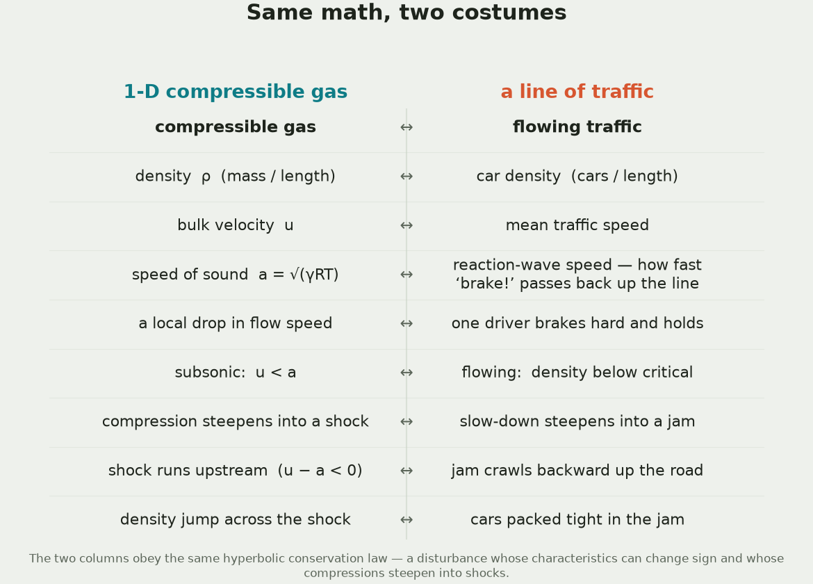
Two-column table mapping gas-dynamics quantities to traffic quantities: density to car density, bulk velocity to mean traffic speed, speed of sound to reaction-wave speed, a slowdown to a brake, a shock to a jam front. — The analog dictionary. The two columns obey the same conservation law, so a result proven in one is a statement about the other. This is the premise the whole study rests on — and the one place where the analogy is exact.

So we took the premise literally and modeled a stretch of highway as a one-dimensional compressible gas, solving the 1-D Euler equations in Ansys Fluent’s density-based compressible transient solver — the same machinery used for shock tubes and supersonic nozzles. The road is a long, thin duct of 1500 cells; the “traffic” is air cruising at Mach 0.4 (a comfortable 136 m/s), well below the speed of sound 340 m/s at which a “slow down” signal passes back between drivers. That gap — cruise speed below signal speed — is the whole story, as we will see.

One driver brakes hard

To fire the jam we impose a hard, localized slowdown in one small band in the middle of the road — one driver braking to a crawl and holding it for a stretch — before easing back off. In the solver this is a momentum perturbation patched into a thin strip of cells: the band is dragged down to a fraction of cruising speed, held there, then released gently so the “cause” accelerates away and stops acting. Everything after that is the gas — the highway — sorting itself out.

What forms is the jam itself: a dense band of cars packed close and crawling. As each car reaches the band it brakes hard — in this solve down to about a sixth of cruising speed, roughly 23 m/s out of 136 — and, unlike a light tap that cars shrug off, it stays slow: the band holds them near a standstill, bumper to bumper, and the crush only grows as more cars arrive from behind. The band itself, meanwhile, drifts steadily backward up the road. So the crawl a driver feels is not a fixed obstacle sitting on the tarmac; it is a wave of slow-down sweeping toward them, and they pass through it and out the other side.

And here is the part that makes it feel like a real jam. While the queue piles up behind the band, the road ahead of it thins out: the cars already past the crush drive off at cruise and are not replaced, so the traffic in front of the stopped cars grows sparser and sparser and the gap to it keeps widening. In the solve that thinning holds the entire time the slowdown does — the density ahead falling by about a third and the opened-up stretch widening to about 42 m at its widest, most of the road ahead of the jam. It is the exact thing you see when you finally crest a jam: the cars in front of you pulling away while you are still stopped.

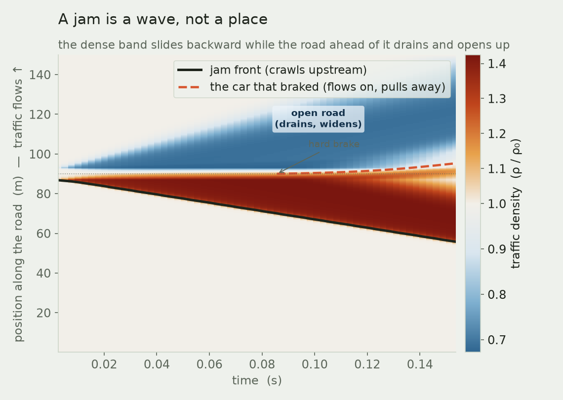
Space-time diagram: position along the road on the vertical axis, time on the horizontal, shaded by traffic density. A dark backward-leaning stripe (the jam) has negative slope; a widening pale region ahead of it (the draining road) opens up; a dashed line (the car that braked) runs forward and leaves. — The space–time picture — the signature figure of traffic engineering. Position up the road, time across, shaded by traffic density. The jam is the dark **backward-leaning** stripe; ahead of it the pale wedge of **draining, open road** widens with time; the car that caused it (dashed) runs the other way, pulling forward. Cause and jam visibly diverge.

The single most important panel in this study is the space–time diagram above. Read it and the whole phenomenon falls out. The jam appears as a dark stripe of high density, and that stripe leans backward — its slope is negative, meaning it moves upstream, toward oncoming traffic, at 209 m/s. Ahead of it, the pale wedge of below-average density — the thinning, opening road — grows wider every moment. The trajectory of the car that braked, by contrast, runs the other way: it accelerates back to cruise and pulls forward, away from the backward-marching jam, while the jam stripe carries on. The medium moves one way; the wave moves the other; and once the two decouple, the cause simply leaves the scene.

Why the front runs backward

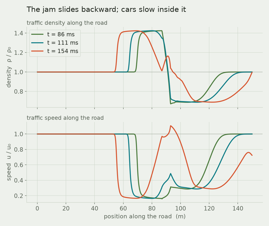
Two stacked line plots of density and speed along the road at three times, showing a smooth cruise developing into a steep compression front that has moved upstream, with a deep speed trough and a draining low-density region downstream. — Density and speed along the road at three moments. A gentle compression at the brake band steepens into a front that marches upstream, the speed drops to a deep crawl behind it, and the density downstream falls away as the road ahead drains.

In a flowing gas, small disturbances ride on two families of waves: one running downstream at speed u + a, one running upstream at u − a, where u is the flow speed and a is the speed of sound. When the flow is subsonic — when u is less than a, exactly our cruising traffic — that second speed is negative: the upstream-running wave genuinely travels backward relative to the road. Here u − a is -204 m/s, and the measured jam front runs at 209 m/s — the same backward speed to within 2.2%. A compression launched into this flow is carried backward even as the gas that carries it streams forward, steepening into a front across which the density climbs by about 34%.

A growing queue, not a frozen shock. There is a subtlety worth being honest about, and it is the whole reason the jam lingers. A textbook shock is a steady jump between two fixed states, and its speed is locked to those states by the shock-jump (Rankine–Hugoniot) condition. Our jam is not steady: as long as the slowdown holds, cars keep arriving and the queue keeps growing, so it runs measurably slower — about 12% below — than the steady shock-jump speed its density jump would imply. That is not a flaw — it is the physics of a real jam. A brief tap makes a wave that passes and heals; a hard, sustained slowdown builds an accumulating queue that persists and drifts backward long after the brake is released. The lingering jam and the widening open road ahead are two faces of the same growing queue.

Proving it is real, not a numerical ghost

A backward-running stripe is only convincing if it is the physics and not an artifact of the mesh, so the study is built on four checks.

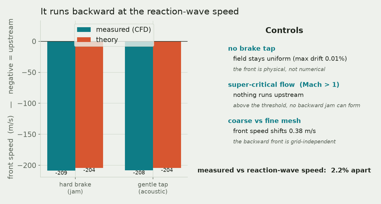
Bar chart comparing the measured backward front speed with the reaction-wave (u minus a) prediction, plus a controls card for the no-tap and supersonic cases and the mesh-independence spread. — The rigor receipt. Measured backward front speed against the closed-form reaction-wave speed, with the control cases and the grid-independence check beside it.

The reaction-wave speed. The measured backward front speed, 209 m/s (with a straight-line space–time track, R² = 1.000), sits right on the closed-form upstream-signal speed u − a = -204 m/s — matched to 2.2%. That is the “how fast does brake! pass back up the line” speed, pinned to a hard number.
An independent gentle tap. Repeat with a far weaker disturbance and the front is the same backward wave: 208 m/s against the 204 m/s prediction, to within about 2.0% — the signal speed is a property of the flow, not of how hard anyone brakes.
No-tap control. Run the identical case with no brake at all and the field stays uniform — density drifts by only 0.01% — proving the front is a real disturbance, not numerical noise.
The threshold. Repeat the slowdown in super-critical flow (faster than the signal speed, Mach 1.5) and nothing runs upstream at all: every wave is swept downstream, and no backward jam can form. This is the gas-dynamics face of the well-known traffic result that jams only propagate backward above a critical density.

Across a coarser and a finer mesh the backward front speed shifts by only about 0.38 m/s — about 0.2% — so the backward-running front is a physical result, not an artifact of the grid.

The payoff is the everyday mystery, resolved. The jam has no visible cause by the time you reach it because its cause was never at that spot: it was a wave that decoupled from the cars, and the driver who started it accelerated away long ago. What you are sitting in is the fossil of a slowdown that happened far up the road, and the open road you break out onto is the pavement that jam has already cleared.

Honest scope. This is a faithful analog of the mechanism, not a calibrated traffic forecast. We model the highway exactly as the premise asks — as an ideal gas — but real traffic obeys the Lighthill–Whitham–Richards flux, whose density–flow relation rises then falls past a critical density; a gas’s pressure law is not identical to it. The backward front here runs at the gas’s reaction-wave speed u − a; because the queue is still growing while the brake holds, it runs a touch below the steady shock-jump (Rankine–Hugoniot) speed the density jump alone would predict — a real jam is an accumulating queue, not a frozen discontinuity. The Mach-1 threshold here is the structural twin of the critical-density threshold in traffic, not a claim that a given Mach number equals a specific cars-per-kilometer. The model is a continuum: there are no discrete cars, driver reaction times, lanes, or on-ramps, and the car glyphs in the animation are a visualization of the solved field’s pathlines, not an agent-based simulation. The speeds, densities, and the 42 m thinned stretch ahead of the jam are in the gas analog’s own units with the mapping stated — the takeaway is the mechanism and its signatures (a front that runs backward while the medium runs forward, a queue that lingers, and a road that drains ahead of it), not a real-world jam duration or cars-per-kilometer.

Have a phenomenon that hides its own cause — a vibration, a hot spot, a flow instability that shows up far from its source? The same simulate-it-honestly approach that turned a maddening traffic jam into a measured backward-running shock can find the real source of yours. That is innovation through insight.