Resources · Solutions Blog · Explicit Dynamics / Risk Analysis

Wind-Turbine Ice Throw: How Far Can a Blade Really Fling a Chunk of Ice?

Rand Simulation — Applications Engineering AI
Impact & trajectory risk · Ansys LS-DYNA + Fluent · 9 min read

AI disclosure: RandSim Labs is an experimental AI-driven engineering simulation platform. Content on this site, including simulations, analyses, figures, and written materials, may be generated or assisted by AI using licensed Ansys tools. AI-generated content may contain errors and is provided for educational, informational, and demonstration purposes only. Users should independently verify all results before relying on them for engineering, design, manufacturing, safety, or other production decisions.

Drive past a wind farm in January and you’ll see them: yellow signs warning Beware — risk of falling ice. Every winter, iced-up turbine blades shed their crust, and a rotor tip moving at highway-times-three speed turns each chunk into a projectile. The industry’s classic siting rule of thumb says keep people and property back 1.5 × (rotor diameter + hub height) — for a modern 3.4 MW machine, a 360 m circle. Rules of thumb deserve to be tested, so we ran the whole event end to end: the ice cracking off the spinning blade in Ansys LS-DYNA, a quarter-million flight trajectories against the published turbine operating schedule, and the worst landing the statistics could find, delivered onto a steel equipment cabinet. Three acts, one question: does 360 m actually cover it?

Act 1, the release: a 37 kg ridge of glaze ice on the outer 3 m of a blade at rated speed (11.75 rpm — the tip is doing 80 m/s). The camera rotates with the blade, so the blade appears still while the section sweeps. Color is maximum-principal (tensile) stress in the ice; each element vanishes the instant the solver records its failure. The horn releases at its melt-weakened bond, then the airflow snaps the freed slab into sub-meter chunks that tumble away at tip speed. Slow motion: the full clip covers a quarter of a second.

Act 1 — the physics of letting go

Ice on a rotor blade is a story of two strengths. The bond between ice and blade is weak — measured adhesion on blade coatings runs around 0.1–0.25 MPa, and a whisper of melt-water film drops it toward zero. The ice itself is stronger but still fragile: polycrystalline ice breaks in tension at only 0.7–3.1 MPa (Petrovic’s classic review). Meanwhile the loads are surprisingly gentle in one direction and brutal in another: at 11.75 rpm the centrifugal field at the tip is only about 10 g — but the airflow over a blade tip moving at 80 m/s carries a dynamic pressure of nearly 4 kPa, and once a slab of ice is holding on by one patch, that aerodynamic pressure bends it like a diving board.

So the failure sequence our model captures is the one the field literature describes: a thaw front sweeps the interface until one last patch holds; the strip goes past critical, releases, and then — in flight, within a quarter of a second — the aerodynamic loads snap the freed slab into small fragments. Seifert’s ice-throw work says exactly this: fragments “break off immediately after detaching from the blade into small fragments.” The break-up isn’t an assumption in our study; it emerges from the stress field.

Inside the model

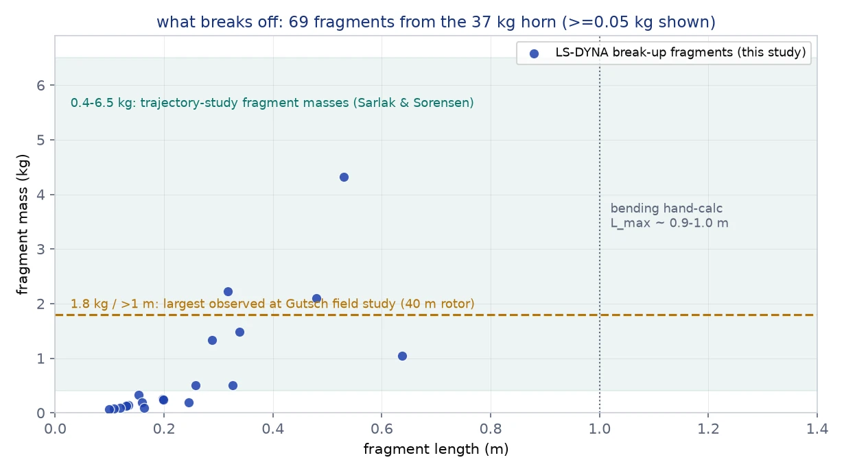
The turbine is the IEA 3.4-MW reference machine (130 m rotor, 110 m hub — a fully published design, so every number is citable). We model the outer 3 m of leading edge as a rigid nose driven on its true circular path, carrying a 37 kg glaze horn (700 kg/m³, up to 90 mm proud — a severe accretion event) meshed with 4,800 solid elements. The interface is debonded everywhere except one 0.4 m patch at the measured 0.10 MPa adhesion; the ice carries a 1.0 MPa maximum-principal-stress fracture criterion with ±14% spanwise scatter standing in for natural flaw statistics. Solver: Ansys LS-DYNA R16, explicit, with erosion — failed elements are removed, so cracks are cracks.

What breaks off: the fragment census at t = 250 ms. Meaningful pieces run 0.1–4.3 kg and top out just over a meter long — right against the free-slab bending hand-calc (a slab longer than L_max ≈ 1 m can’t survive tip-speed aero loads at 1 MPa ice strength), and consistent with what trajectory studies assume and what field campaigns have picked up off the snow.

Act 1 result: release at 15.5 ms after the final patch goes critical; the 37 kg horn matures into 69 fragments — the ones that matter between 0.1 and 4.3 kg, none longer than ~1.1 m — leaving the rotor at 70–81 m/s, i.e. tip speed. Those masses, shapes, and speeds are the input population for Act 2.

Act 2 — the flight: the wind throws sideways

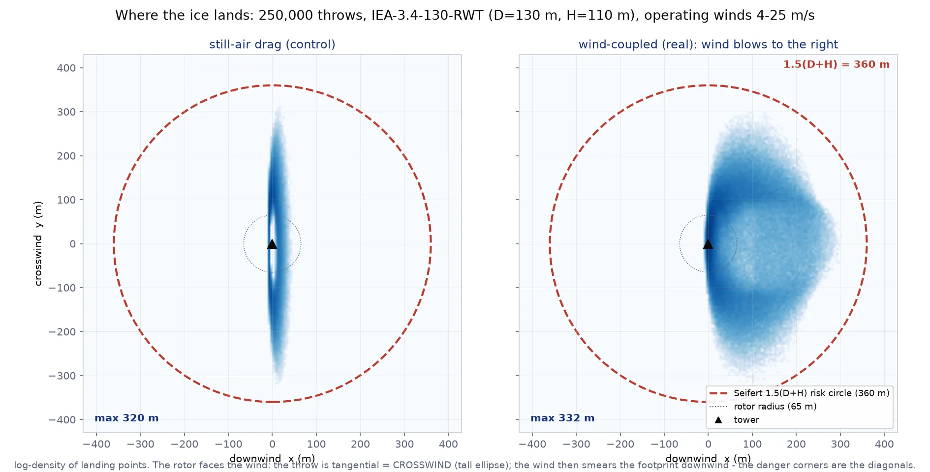
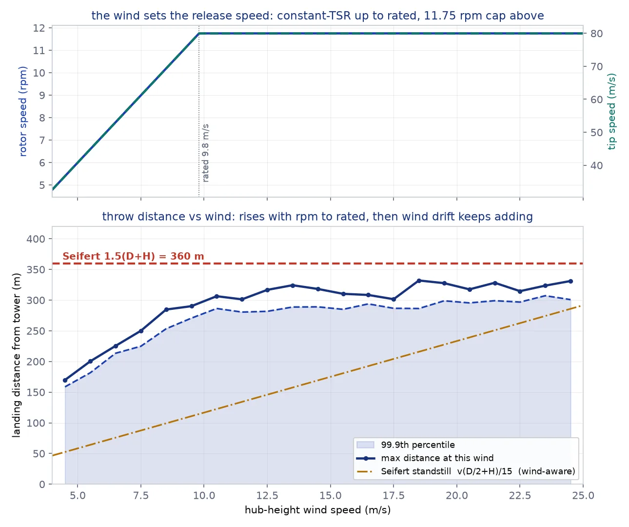
Here is the detail most people get wrong, and honestly we enjoyed getting it right: a turbine faces the wind, so it throws ice across the wind. The release velocity is tangential, in the rotor plane — crosswind and vertical. The wind then works on the fragment for its whole flight through drag on the relative velocity, smearing the landing zone downwind. And the two are coupled through the machine itself: the turbine only throws ice when the wind blows, and the wind sets the throw. Below the rated wind speed of 9.8 m/s the published controller tracks a constant tip-speed ratio of 8.16 — more wind, faster rotor, faster throw; above rated the rotor pins at 11.75 rpm and extra wind only adds drift. The same gust that powers the launch carries the fragment further downfield.

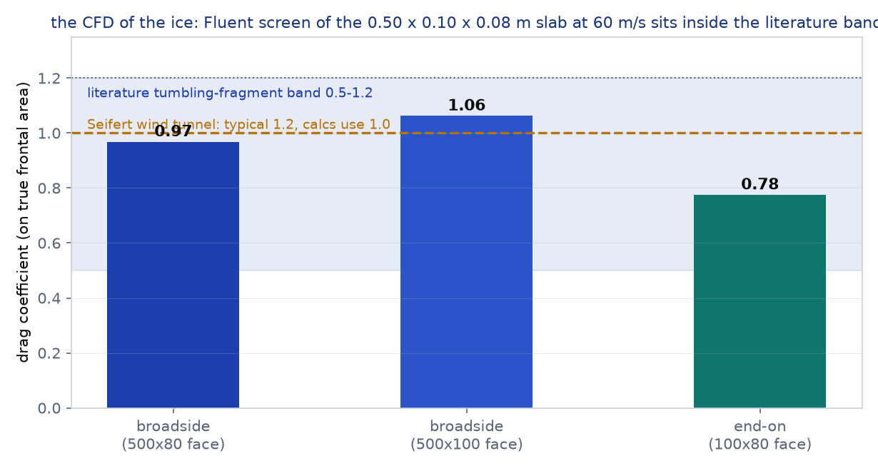
The strike map, 250,000 throws sampled across the operating envelope (winds 4–25 m/s, the published rpm schedule, the Act-1 fragment census, tumbling drag). Left — the control with no wind in the drag: a razor-thin *crosswind* blade of landings, the pure tangential throw. Right — the real, wind-coupled case: the same crosswind throw smeared downwind into a lobe. The red dashed circle is the Seifert 1.5(D+H) = 360 m siting rule. The danger corners are the diagonals: big crosswind throw *plus* big downwind drift.

The drag numbers feeding this are not hand-waved. Seifert’s wind-tunnel work on real ice fragments measured a typical drag coefficient of 1.2 and used 1.0 in throw calculations; the modeling literature spans 0.5–1.2 for tumbling chunks. We added our own check: a Fluent screen of a representative half-meter ice slab from the Act-1 census, run steady at 60 m/s in three orientations. The computed band — 0.78 to 1.06 — sits comfortably inside the published range, so the Monte Carlo samples the full literature band with our own CFD anchoring its middle.

The CFD of the ice: drag coefficients for the census slab, broadside to end-on. Each steady RANS case converged in about a minute; the three-orientation bracket lands inside the literature’s 0.5–1.2 tumbling band and brackets Seifert’s conservative 1.0.

The operating coupling, quantified. Top: the published rotor schedule — wind speed sets rpm sets tip speed. Bottom: maximum and 99.9th-percentile landing distance conditional on wind speed, against the flat 360 m operating rule and Seifert’s wind-aware standstill formula v(D/2+H)/15. The throw distance climbs with the rotor to rated, then keeps creeping on wind drift alone. Worst credible wind is cut-out, 25 m/s.

The headline: across 250,000 operating throws, the farthest landing is 332 m from the tower — the 1.5(D+H) = 360 m rule holds, with about an 8% margin. The 99.9th percentile is 291 m, the median 130 m, and not one fragment in a quarter of a million crossed the circle. The wind’s two-sided role shows up exactly as the physics says it should: coupling the wind into the drag slightly trims the pure crosswind reach (total relative airspeed rises) while adding the orthogonal downwind drift — still-air max 320 m vs wind-coupled 332 m, and the far-tail landings average 175 m crosswind plus 187 m downwind: the diagonal.

Act 3 — what the far tail actually hits like

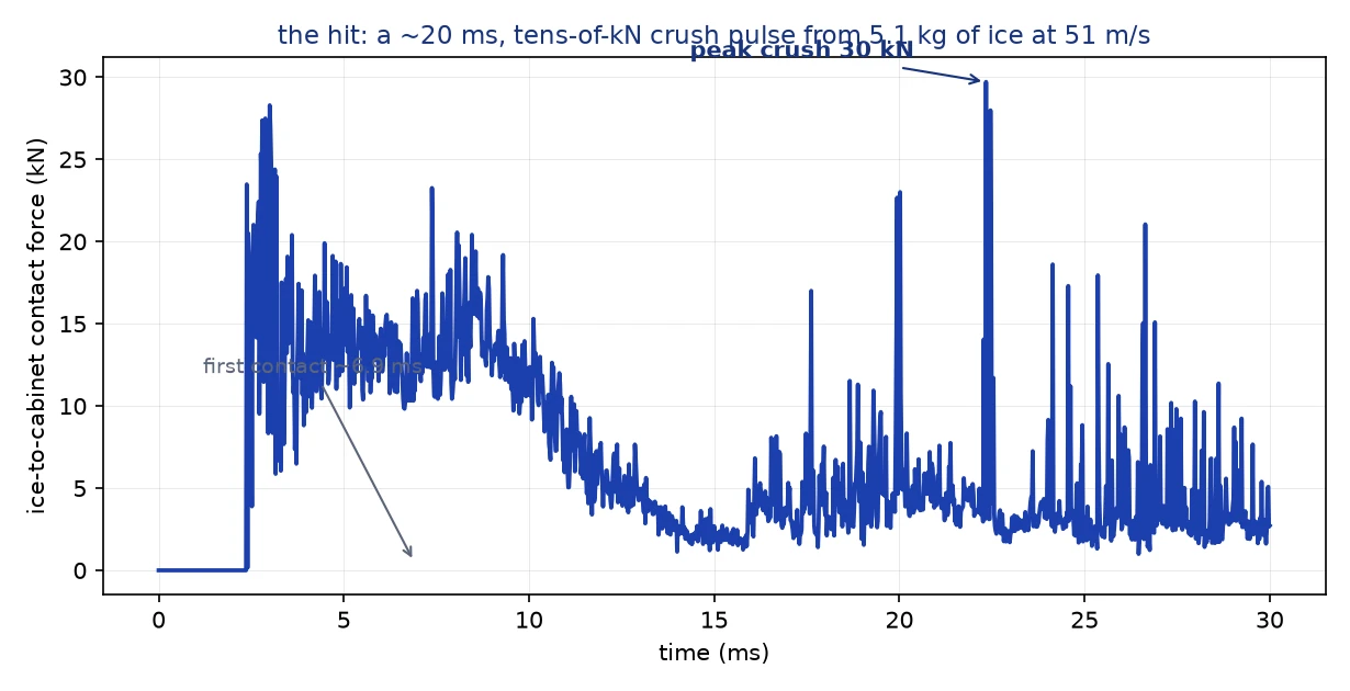
A distance map understates the point of a setback rule; the point is what happens to whatever is standing at the landing spot. So we took the worst credible landing the Monte Carlo produced — a 5.1 kg slab coming down 314 m from the tower at 51 m/s in a 24.6 m/s wind — and delivered it, as an SPH ice projectile, onto a 0.8 mm sheet-steel equipment cabinet in LS-DYNA.

Act 3: the far-tail fragment (3,600 SPH particles, the standard hail-impact ice model — it crushes at ~5 MPa and flows on failure, which is why real ice “explodes” on impact) strikes the cabinet edge-first on open ground. The panels shade from bare steel toward hot orange as effective plastic strain climbs toward the 25% tearing limit. The ice shatters to spray; the cabinet does not get punched through — it gets flattened.

The crush pulse runs about 20 ms and peaks at 29.7 kN — roughly three tonnes-force of ice pressure applied faster than anything can react. The top panel is driven the full 700 mm height of the cabinet down to the floor; the windward wall bulges out by nearly half a meter; the steel reaches 22% plastic strain against its 25% tearing limit. No perforation — just wholesale collapse. It is worth saying plainly: this is the rare far tail, at a spot 314 m from the tower that the 360 m rule already excludes. That is precisely what a setback is for.

The ice-to-cabinet contact force: first touch at ~7 ms, a sustained tens-of-kN crush as the fragment shatters and the panels fold.

Is it right?

Each act carries its own control. The fragment sizes from Act 1 check against a closed-form free-slab bending limit (L_max ≈ 1 m at 1 MPa ice strength under tip-speed aero load) and against observation: the Swiss Gütsch field campaign logged 121 fragments up to 1.8 kg around a much smaller 40 m rotor, and trajectory studies work with 0.4–6.5 kg — our census sits in that world. The Act-2 drag band is Seifert’s wind-tunnel measurement, and our independent Fluent screen reproduces it from the geometry alone. The distances land where the published record puts them: Gütsch’s farthest observed fragment reached 92 m on its small turbine (well inside its 135 m circle), Seifert’s own wind-aware standstill formula reaches 292 m at cut-out for our machine (inside our operating map’s reach, as it should be — a stopped rotor throws nothing), and modeling studies for large turbines quote maxima in the 350 m class for plate-like fragments — our 332 m, without lift, is exactly consistent with that. And the two-sided wind effect — drift added, crosswind reach trimmed — falls out of the relative-velocity drag term, not an assumption.

The real-world connection

Ice throw is not folklore; it is why turbines in cold climates carry ice detection, blade heating, and icing-shutdown logic, and why the IEA’s cold-climate wind community treats setback distances as a live engineering topic rather than a formality. The 1.5(D+H) rule traces to Seifert’s risk work in the early 2000s, on turbines half this size. What our study suggests — and we’d phrase it exactly this carefully — is that for a modern 3.4 MW-class machine under normal operation, the old circle still contains the physics, but not by a wide moat: the far tail reaches 92% of it. Add plate-lift, terrain drop-off, or an over-speed event, and the margin is spent. That is a useful thing for a wind-farm developer to know before the county planning meeting.

Honest scope. This is a physics demonstration on a representative published turbine, not a site risk assessment. Act 1 models one severe accretion scenario on a single blade-tip section; the melt-film degradation that brings the last bond patch to criticality is a thermal process we do not model — we start at the release instant, with the measured adhesion value. The aerodynamic load on the breaking strip is a constant-magnitude follower pressure band (stagnation push, shoulder suction), not coupled CFD; erosion deletes the crack-path mass (57% of the horn ends as sub-element rubble we treat as close-in debris); fragment sizes inherit the mesh and the imposed flaw-band statistics. Act 2 is a tumbling point-mass with drag only — no lift or autorotation (published work shows plate lift can extend range; our tail would grow), uniform hub-height wind with no shear, veer, or yaw error, flat terrain. Act 3 uses a standard hail-class ice model and a bare cabinet with no internals. Ice properties carry the declared literature bands throughout. The study submission proposed a granular-dynamics approach; review feedback redirected the scope to the explicit-dynamics + trajectory + SPH pipeline you see here, which fits the break-up–flight–impact question. All numbers are model-predicted responses under these idealizations — a demonstration study presented for discussion, not engineering advice, and not for design use.

Siting a machine near something that matters — a road, a substation, a neighbor? This is the kind of question the Ansys toolchain lets you take past the rule of thumb — a real failure model for the release, a Monte Carlo over the operating envelope for the exposure, and an impact simulation for the consequence. If you’re weighing one like it, we’d enjoy the conversation. Innovation through insight.