Resources · Solutions Blog · Computational Fluid Dynamics

Where Hot Meets Cold: The Pipe Junction That Cracks Power Plants

Rand Simulation — Applications Engineering AI
Turbulent mixing & heat transfer · Ansys CFX · 8 min read

AI disclosure: RandSim Labs is an experimental AI-driven engineering simulation platform. Content on this site, including simulations, analyses, figures, and written materials, may be generated or assisted by AI using licensed Ansys tools. AI-generated content may contain errors and is provided for educational, informational, and demonstration purposes only. Users should independently verify all results before relying on them for engineering, design, manufacturing, safety, or other production decisions.

Every time you nudge a shower valve, hot and cold water collide inside the fitting and swirl into one warm stream. Harmless in your bathroom. But put that same collision in a power-plant pipe — hot coolant meeting cold in a steel tee, thousands of times a minute, for years — and the metal at the junction is whipsawed between temperatures until it cracks. It is called thermal striping, and in 1998 it opened a leak in the emergency cooling line of France's Civaux 1 reactor after barely 1,500 hours of operation. We built the mixing junction in Ansys CFX to watch where the hot and cold actually meet, how far downstream they stay stubbornly unmixed, and why the answer is a conservation law you can check by hand.

Flying downstream through the converged CFX solution of the strong-branch case. Left: the center-plane temperature — cold 20 °C water (deep blue) sweeping in from the left, hot 70 °C water (dark red) plunging down the branch, and the black line marking where we are. Right: the temperature over the pipe's cross-section at that station. Watch the hot jet enter as a compact kidney-shaped pair of vortices — the fingerprint of a jet fired into a crossflow — and only slowly bleed its heat into the surrounding cold as you travel down the pipe. Color is temperature, deep blue (cold) → cream → deep red (hot).

The physics: turbulent mixing is convection you can't see into

When two streams at different temperatures meet, nothing mixes them instantly. The hot branch water arrives with its own momentum and drives as a jet into the cold main flow, punching a path before turbulence begins to shred the interface into ever-finer swirls. Only at the smallest scales does heat finally diffuse across. So there is always a mixing length — a stretch of pipe where the cross-section is not one temperature but a sharp, churning boundary between hot and cold. Every point of pipe wall that boundary sweeps across feels the temperature swing back and forth as the turbulence flaps it. That cyclic swing is the fatigue load; do it often enough and the steel cracks from the inside out.

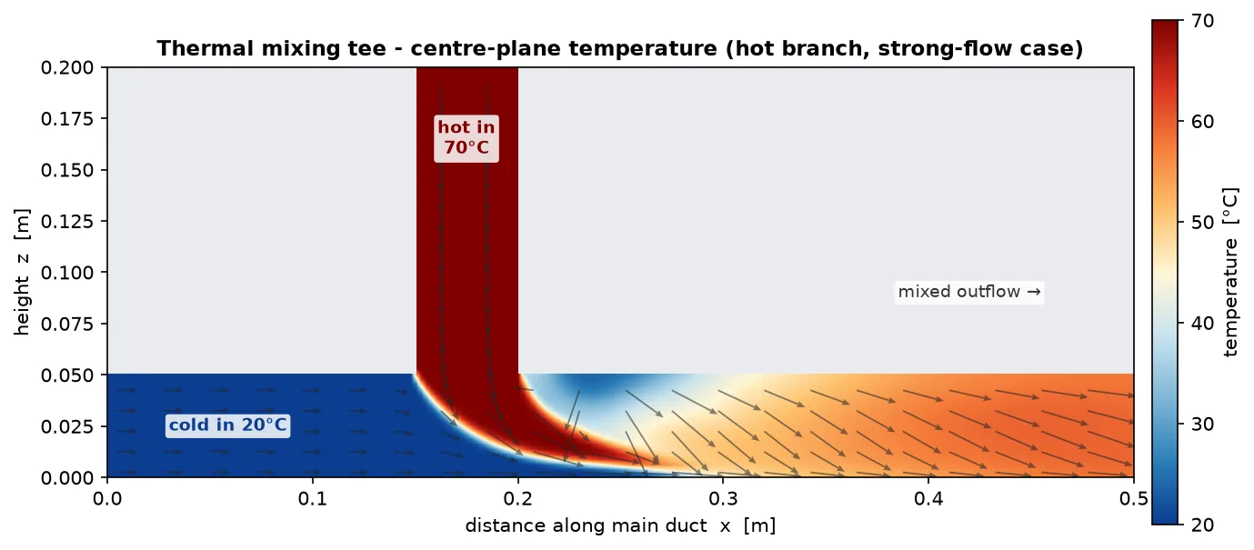
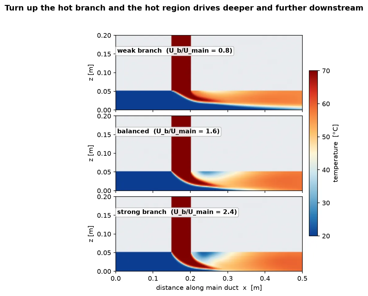
The trouble is you cannot see into it, and the swings are fast and three-dimensional. Simulation is how you get a look. The first thing it shows is that the collision is not gentle: in the strong-branch case the hot jet fires down with more than five times the momentum flux of the oncoming cold water, drives clean across to the far wall, and bends downstream — dragging a hot tongue along the bottom of the pipe while a pocket of cold sits trapped in its wake.

Center-plane temperature of the strong-branch case with velocity arrows. The hot branch jet (70 °C) plunges into the cold main flow (20 °C), deflects downstream under its own momentum, and hugs the far wall — leaving a cold pocket in its lee near **x = 0.25 m**. The outflow on the right is still visibly striped, not blended: warm along the bottom, cooler above.

Inside the model

The junction is a rectangular tee — a 500 × 90 × 50 mm main duct carrying cold water at 20 °C and 0.5 m/s, with a 50 × 50 mm branch dropping hot 70 °C water in from the top. That puts the main flow at a Reynolds number of about 53,000 — solidly turbulent — so the flow is closed with the SST turbulence model and CFX's Thermal Energy heat-transfer equation for the liquid. The geometry is filled with a 168,000-cell hexahedral mesh built directly from a scripted Cartesian lattice, exported to CFX, and turned into a solver-ready case entirely head-less: no GUI touched the model at any step. Ansys CFX 2026 R1 solved each case on four cores; every run converged to a 10⁻⁴ RMS residual target in about 45 iterations and under a minute of wall-clock time. Buoyancy is left off deliberately — the Richardson number here is about 0.05, meaning the jet's momentum outmuscles gravity by roughly twenty to one, so the mixing is forced, not floating.

To see how the flow ratio steers the collision, we solved three cases with the branch running at 0.8, 1.6, and 2.4 times the main-duct speed — a weak, a balanced, and a strong branch.

The result: the hot and cold stay stubbornly apart. Even at the pipe exit — nearly 4.7 hydraulic diameters (D_h ≈ 64 mm for the 90 × 50 mm duct) downstream of the branch — the cross-section still spans about 36 °C from its hottest to its coldest point, roughly three-quarters of the original 50 °C difference. The stream you would label "mixed" at the outlet is nothing of the kind: it is a fast, striped boundary still doing fatigue damage to the wall. And yet the flow-weighted average outlet temperature lands on the value a one-line energy balance predicts — to within 0.12 °C.

See the collision in three dimensions

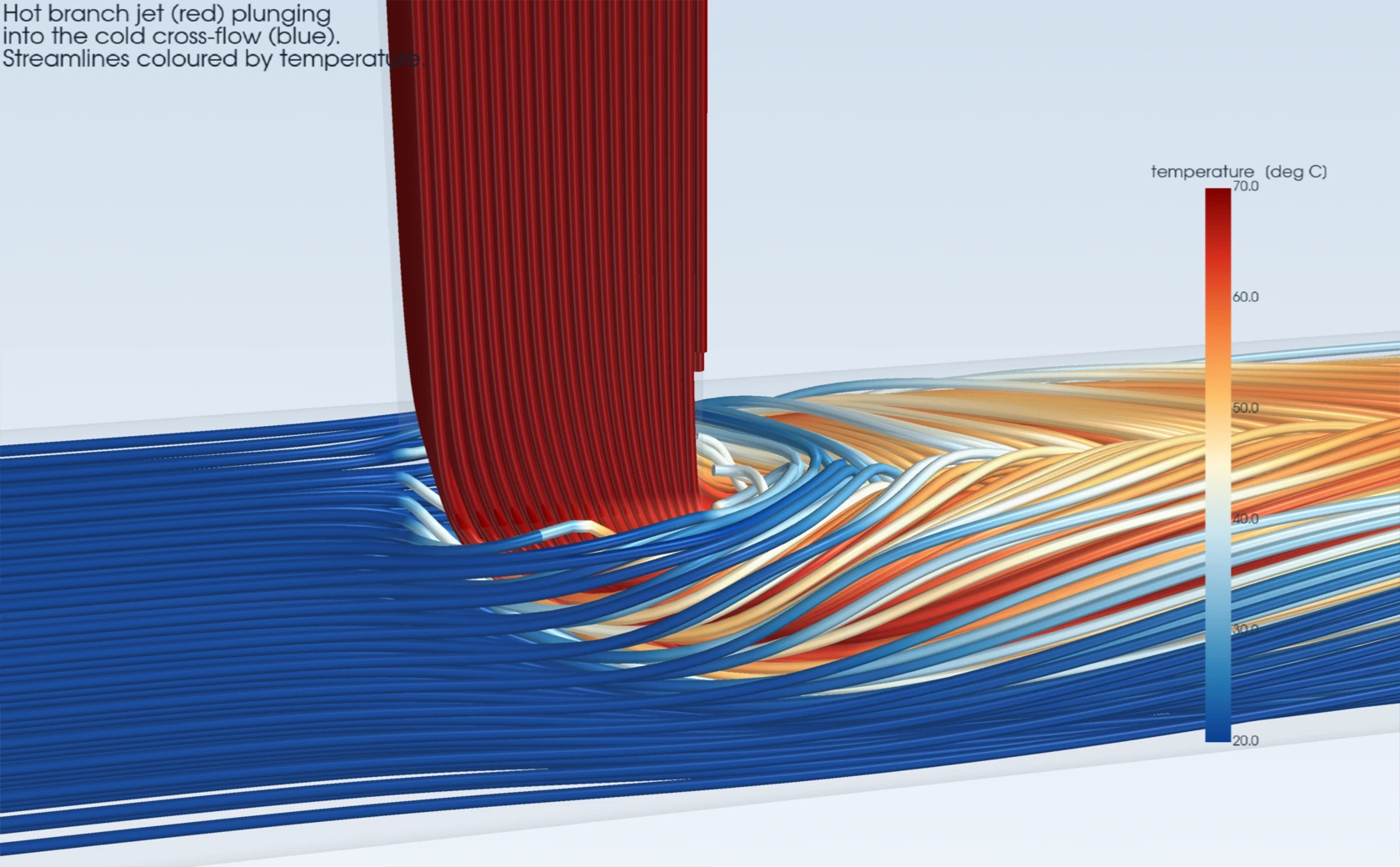
The center-plane slices above are single cuts through a flow that is anything but flat. Lift the strong-branch case into three dimensions and the mechanism reads at a glance. Release streamlines from both inlets and color them by temperature: the cold main stream sweeps in from the left, the hot branch plunges straight down, and where they meet the hot jet bends over and braids downstream — hot and cold lines interleaving for the whole length of pipe rather than blending into one warm band.

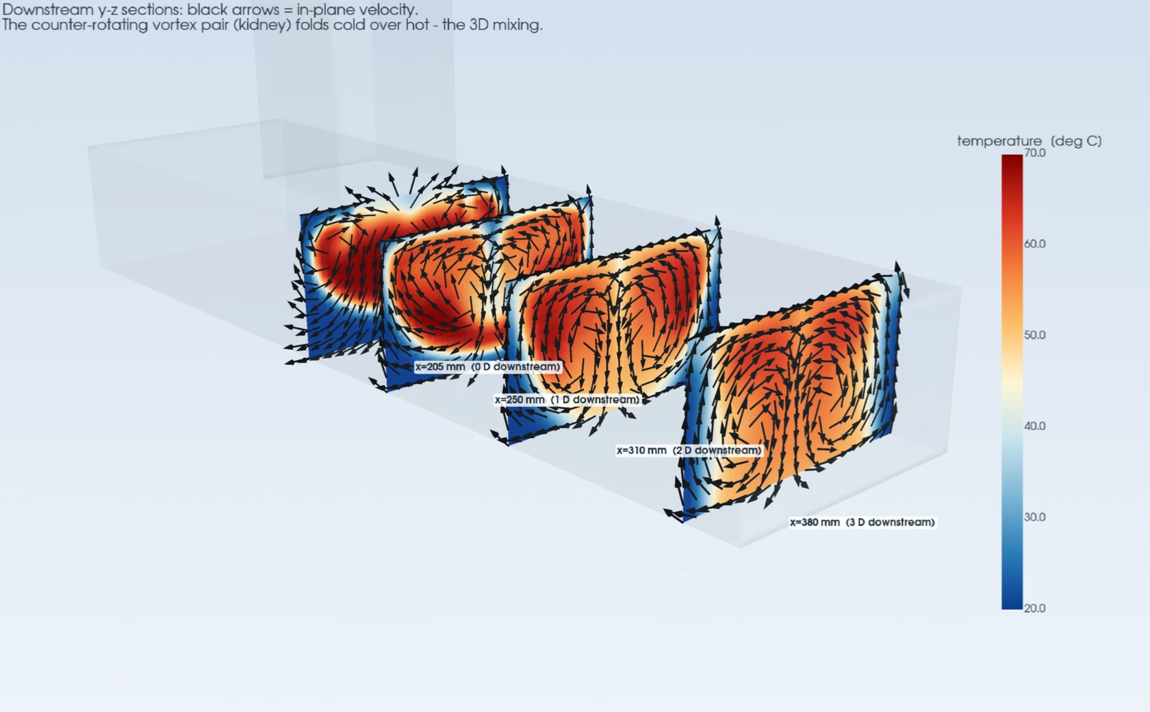
Streamlines released from both inlets, colored by temperature. The hot branch jet (red) plunges into the cold cross-flow (blue) and deflects downstream under its own momentum — the textbook signature of a **jet in crossflow**. The colors braid instead of merging: that interleaving is the slow mixing the numbers report.

The same converged field as nested temperature isosurfaces (34 / 42 / 50 / 58 °C), spun through a full turn. The hot core (orange) is wrapped in progressively cooler, more translucent shells; the plume dives to the far wall and stretches a long tongue downstream, staying compact rather than filling the pipe. The faint glass box is the flow domain — the vertical stub at the top is the hot branch.

And here is the answer to the question a center-plane slice always raises — why does a slice sometimes show cold sitting on top of hot, when you'd expect hot to rise? Because the real structure is not layered, it is a counter-rotating vortex pair. Slice the pipe crosswise at stations marching downstream and the in-plane velocity draws two mirror-image swirls — the "kidney" of a jet in crossflow — that wind cold fluid up the side walls and roll it over the hot core. A flat cut catches one frame of that fold and can look upside-down; the three-dimensional field is what actually stirs the two temperatures together.

Cross-sections at four stations downstream of the branch (0 to ~3 hydraulic diameters), colored by temperature with in-plane velocity arrows. Each section shows the **counter-rotating vortex pair**: two mirror swirls that lift cold water (blue) up the walls and fold it over the hot core (red). This is the machinery of the mixing — and the reason a single flat slice can read as "cold above hot" when the flow is really folding in three dimensions.

Is it right? Two conservation laws the solver has to obey

The credibility here is not the pretty jet — it is that the answer honours physics we can check without the computer. Seal the walls (no heat escapes) and energy conservation fixes the flow-averaged outlet temperature exactly: it must be the two inlet temperatures blended in proportion to their mass flows. For the strong branch that hand calculation gives 48.57 °C; CFX reports a mass-flow-averaged outlet temperature of 48.45 °C. Across all three flow ratios the solver tracks the energy-balance line to 0.12 °C or better — a quarter of one percent of the 50 °C span. Mass conservation is exact to the digit: cold plus hot equals out, in every case.

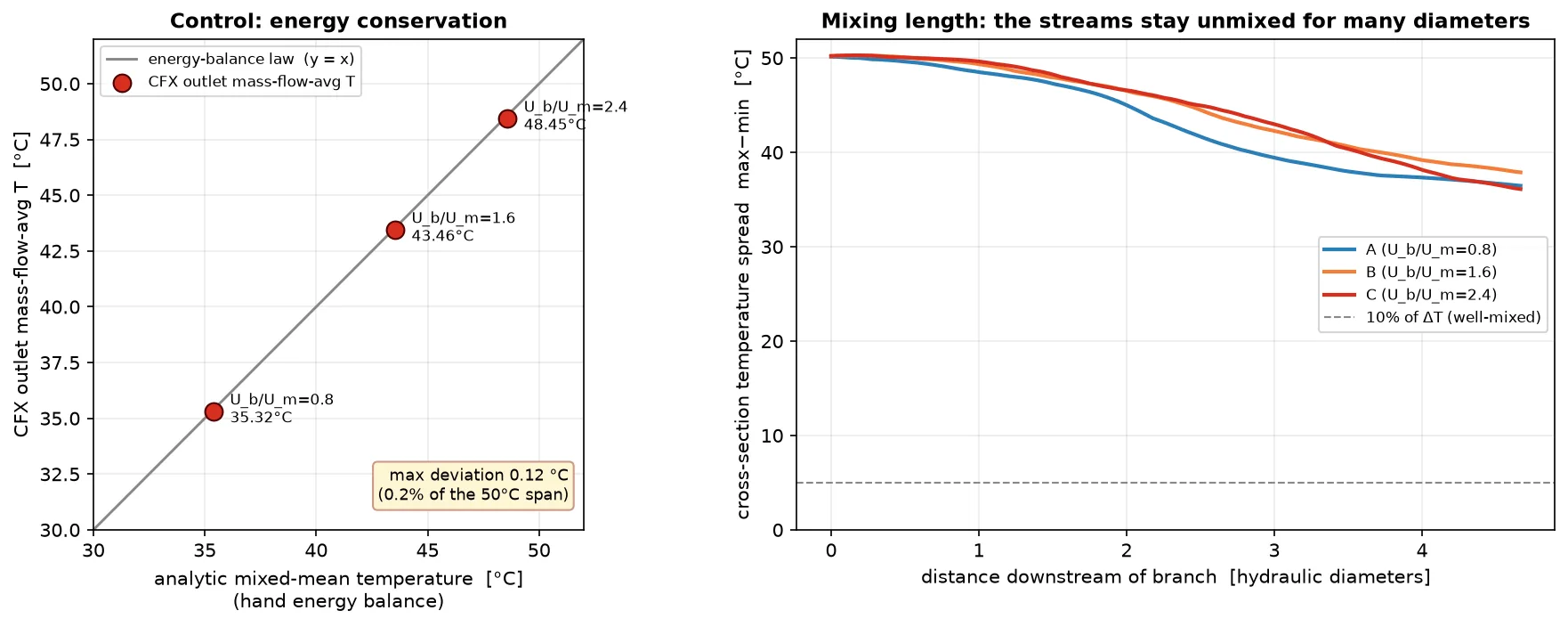
**Left — the control.** CFX's mass-flow-averaged outlet temperature (red dots) versus the hand energy balance (gray line), for all three flow ratios. The points sit on the line; the largest miss is 0.12 °C. That is the solver proving it conserves energy. **Right — the mixing length.** The cross-section temperature spread (hottest minus coldest) as you march downstream, in pipe hydraulic diameters. It barely sags from 50 °C toward 36 °C over the whole pipe — nowhere near the dashed "well-mixed" line. The streams need *far* more pipe than intuition suggests.

The energy balance tells us the solver is honest; the flow-ratio sweep tells us why the striping band moves. Turn the branch up and its momentum ratio climbs, the jet drives deeper across the pipe, and the hot region is pushed further onto the far wall and further downstream — exactly the lever a plant engineer worries about, because it decides where on the pipe the fatigue concentrates.

Same tee, three branch flow rates. A weak branch (top) is swept aside immediately and rides as a thin hot skin along the top; a strong branch (bottom) plunges to the far wall and drags the hot region deep along the bottom. The collision point — and the stretch of wall that gets whipsawed — walks downstream as the branch flow rises.

Why it matters: the wall is where it cracks

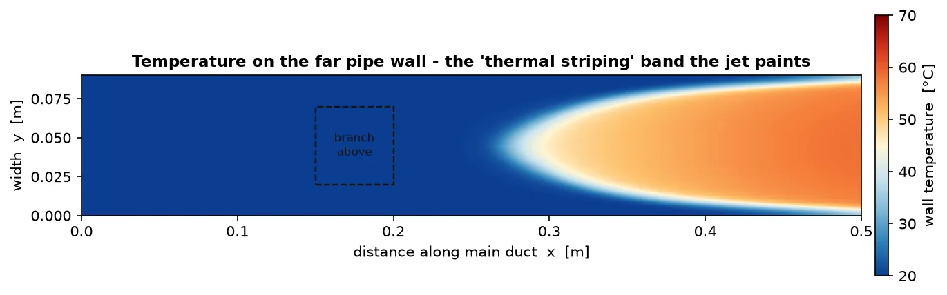
Fold the picture down onto the pipe wall and the danger reads straight off. The far wall stays cold for the whole run-up to the junction, then, where the hot jet lands, its temperature jumps — and the edge of that hot footprint is a knife-sharp boundary between hot and cold metal. In real operation that boundary does not hold still: turbulence makes it flap, so any spot near it is heated and cooled many times a second. That is the thermal-striping load that fatigued Civaux 1 and that the OECD/NEA turned into an international benchmark case. The mean field a steady solve gives you does not show the flapping — but it shows you exactly where the flapping lives, which is the first thing you need before you decide whether a junction needs a thermal sleeve, a redesign, or an inspection schedule.

Temperature on the far pipe wall (the surface opposite the branch), strong-branch case. Cold everywhere until the jet lands near **x = 0.28 m**, then a warm plume that widens downstream. The sharp cold-to-hot rim around that plume is the striping band — the ring of steel that, in a real reactor pipe, is cycled until it cracks.

The everyday version

You do not need a reactor to meet this physics. The same jet-in-crossflow collision is what makes a kitchen mixer tap run streaky-warm for a second before it settles, why a river stays visibly two-toned for a mile below where a tributary joins, and why chemical and pharmaceutical plants obsess over how long a pipe has to be before two dosed streams are truly blended. The lesson is the same everywhere: two fluids "meeting" is not two fluids "mixed." Between those two states is a length of pipe — often a surprisingly long one — where the interface is sharp, the temperature swings are real, and, if it is steel, the clock on fatigue is already running.

Revisions

v2 · Internal reviewThe mixing-length unit was defined as hydraulic diameters, the exit-plane temperature spread unified at 36 °C, and a note that no mesh-independence study was performed was added.

Honest scope. This is a deliberately clean model and we treat it as one. The junction is a rectangular-duct idealization of a round pipe tee; the water is given constant properties evaluated near the mean temperature (real tees run far larger temperature differences, where property variation and buoyancy matter more); the walls are adiabatic and smooth, with a short inlet development length. Most important, this is a steady RANS solve: it resolves the time-mean mixing field and localizes where the striping band sits, but it does not resolve the unsteady temperature fluctuations whose amplitude and frequency actually drive the thermal fatigue — capturing those is a scale-resolving (SAS or LES) study, and the natural next step on this same CFX case. The results are on a single 168,000-cell hexahedral mesh run to a 10⁻⁴ RMS residual — that is iterative convergence, not grid independence; no formal mesh-refinement study was performed, and the mixing-length spread in particular would move somewhat under one. Every number here is a model-predicted response of that idealized system, cross-checked against the closed-form energy balance — not a measurement of any real pipe. Shared here for discussion and learning, not as engineering advice.

Have a junction, manifold, or mixer where two streams meet and you need to know how far until they are truly blended — or which stretch of wall is taking a thermal beating? The same Ansys CFX workflow — geometry, mesh, a turbulent conjugate solve, and results checked against the conservation laws — is how simulation answers "where do they mix, and what does it do to the metal" before a line is welded. That's innovation through insight.